How to use Interval Data |
Top Previous Next |
|
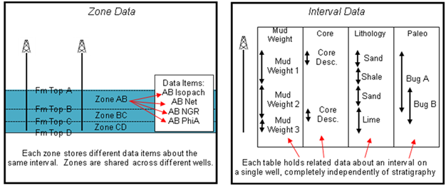
Interval data stores data to a specific depth interval that doesnt fit well with the traditional zone concept, such as data that is too fine (such as core descriptions) or too coarse (such as mud weights or biostratigraphic information) to fit inside two formation tops. The difference between Zones and IntervalsPetra defines a Zone as a specific interval defined by a discrete top and a base. Usually a zones top and base are defined by specific formation tops so that the zone covers a consistent lithostratigraphic unit. Inside each zone, Petra stores a Data Item such as isopach, net pays, or log measurements that relate to that zone. Since zones and their data items are shared across all wells in a project, this method of organizing data makes storing and mapping single-value data for a specific formation much easier. As an example, mapping all the isopach values for a specific formation is much easier when the values are all stored in one common zone data item for each well. Zones are limited, however. Cuttings or core data may actually subdivide a specific zone into several different units based on lithology, color, porosity, or other petrophysical characteristics. Similarly, data such as a mudweight or a biostratigraphic presence can be larger than a single zones definition. Capturing all this information with the traditional zone model is cumbersome as it leads to a proliferation of new, well-specific zones. Intervals, on the other hand, are designed to store information about the wellbore without using zones. The interval concept stores data too fine for the zone concept (such as core and lithologic descriptions) as well as data that exists completely outside the normal stacked strata concept (such as logging runs or mud weights). Interval data also handles data overlapping different formations, such as paleostratigraphic data.
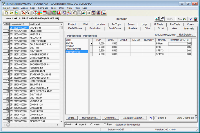
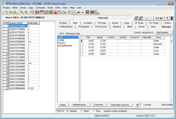
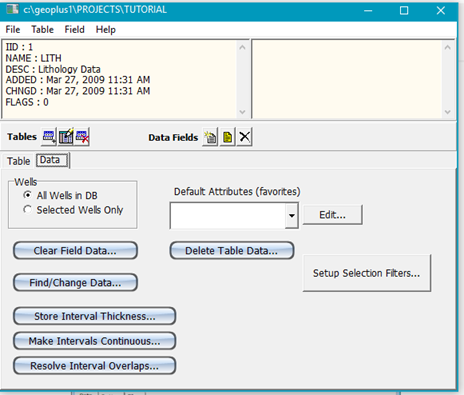
Interval Data BasicsPetra stores interval data in tables and fields similar to a spreadsheet. The table stores related interval data in a spreadsheet, where each interval is stored as a separated row. In the example below, the project has the default tables LITH, CORE, and PALEO. Inside the table, each interval is stored as its own row, and information about that interval is stored in fields, or columns in that row. All tables come with a few fields, TOP, BASE, DATE1, DATE2, QUALITY, and FMNAME, but you can add user-defined fields containing numbers, dates, or text. In addition to the standard fields, the LITH table in the example below contains the field Desc which stores lithologic descriptions. Creating, Modifying, and Deleting tablesAn interval data table stores interval data in a spreadsheet, where each interval is stored as a separated row. Since every interval row in the table shares the same fields (as columns), its a good idea to keep different types of data in different tables. To create, modify, or delete tables in a Petra project, select the Maintenance button on the bottom of the Interval tab on the Main Module.
Creating, Modifying, and Deleting New FieldsIn an interval table, each interval is stored as its own row, and information about that interval is stored in fields, or columns, in that row. To create, modify, or delete fields in a Petra project, select the Maintenance button on the bottom of the Interval tab on the Main Module.
Reordering tables By default, interval tables show up in the order theyre created. Especially in large multi-discipline, multi-user projects with many different kinds of data, its often useful for a user to reorder and filter the interval tables to only show relevant data. To reorder the Interval tables, select the Order... button on the Interval tab on the Main Module. This brings up the Filter Interval Data table Names box. Here, use the > button to bring a single selected table from the Available Internal table List on the left to the Filtered Interval table List on the right. The >> button brings over all available tables. Once on the Filtered Interval table List, use the up and down arrows to change the order of the shown tables. tables at the top of the list will be shown before tables on the bottom of the list. To drop a selected table from the Filtered list, select the < button, and to drop all tables from the filtered list, select the << button. If there are any tables on the Filtered Interval table List, only those tables will be shown.
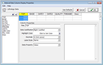
Reordering and Hiding Fields By default, interval fields show up in the order they are created. To reorder the Interval fields, select the desired table and select the Columns... button on the Interval tab on the Main Module (highlighted on the left figure below). This brings up the Interval Data Column Display Properties window. This screen shows the list of the tables available fields on the left, the displayed fields on the upper right, and the selected fields properties are shown in the lower right. This window changes the order of the displayed fields, hide and show specific fields, and changes field properties.
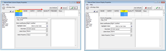
Reorder the specific fieldsTo reorder a field, select the column at the top of the screen and drag it to the desired position. In the example below, the TOP column has been dragged to be before the QUALITY column.
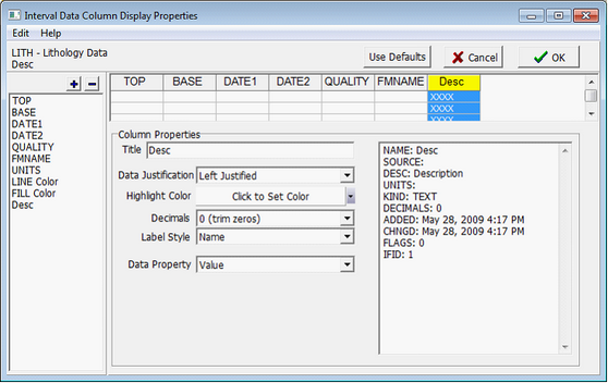
Hide and show specific fieldsTo drop a specific field, select the column at the top of the screen and select the - button. To add a specific field, select the field name from the list on the left side of the window and select the + button. Change the field propertiesThe Column Properties on the lower right shows name, justification, shown decimals, the label style (Name or Name and Units), and the data property (Value or Quality). Changing these settings changes how the selected field will be shown.
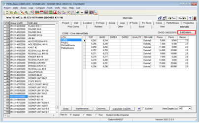
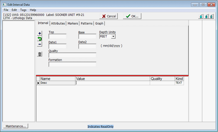
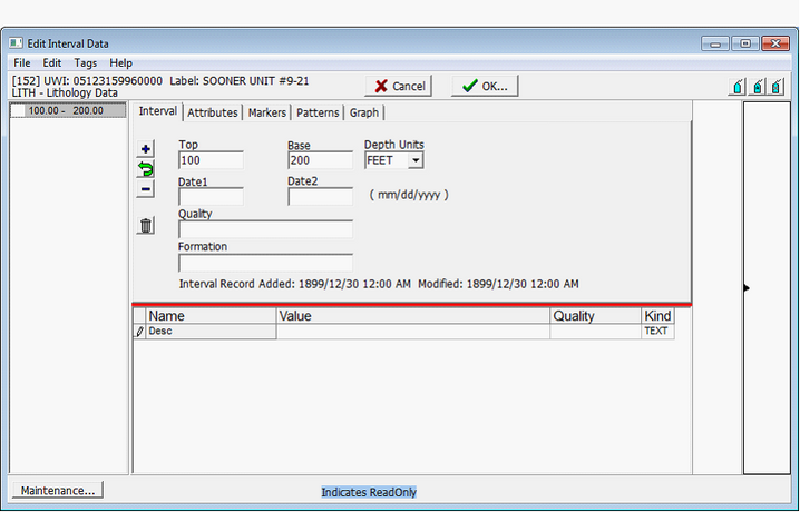
Adding Interval Data New interval data can be brought into Petra either manually or by a tabular data import. Adding New Data ManuallyTo add new intervals manually, first select the correct well in the Main Module. On the Interval tab, select the right interval table. In the example below, the LITH table is selected. Finally, select the Edit details button in the upper right on the Interval tab. This brings up the Edit Interval Data window for the selected interval table. Continuing with the example, the Edit Interval Data window below shows the fields for only the LITH table.
To add a new interval, enter in the Top and Base. Next, select the button to add the interval.
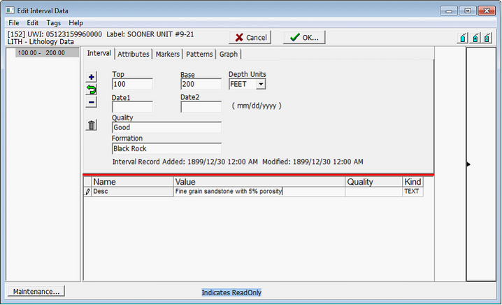
With the interval now added, enter in the remaining interval details and select button to save the changes to the interval. In the example below, the Quality, Formation, and LITH table specific fields are filled in.
To save the changes to the database, select OK. Here, Petra gives the option to save or discard ALL changes made to the selected wells interval table. All the edits to all intervals will be ignored if you select CANCEL. Importing tabular Interval DataDigital data where each row contains information about a discrete interval can be easily imported into Petra. Before attempting to import interval data, check to see if the data has a column dedicated to the UWI/API. Since Petra assigns interval data to specific wells by comparing UW/API numbers, interval data without an identifying API/UWI column cant be imported. The easiest way to remedy this is to simply open the interval data in a spreadsheet program, and add a new column for well UWI/API.
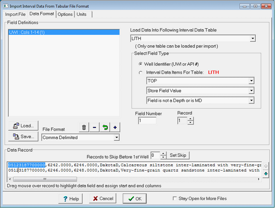
To import new digital interval data, select Project>Import>Import tabular Interval Data on the menu bar at the top of the Main Module. This opens the Import Interval Data from tabular File Format box. Here, select the Open File button and navigate to the interval datas location.
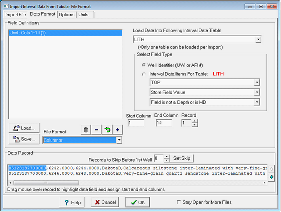
Once the file containing the interval data is opened, Petra switches to the Data Format tab. This tab essentially links the entries in the file to specific kinds of data. The first step is to select the interval data files formatting under File Format. Files can be imported into Petra in one of three formats: Columnar, Comma Delimited, or ~ Delimited. Columnar data organizes data into fixed columns, where Petra imports data based purely on the number of characters from the left. The left screenshot, on the other hand, shows the API number as defined by columns 1 through 14. Comma and ~ delimited data, on the other hand have no fixed column size and are instead separated by a comma or a tilde. With delimited data, Petra imports data based on the Field defined by the delimiter. The example below shows the same UWI/API field defined in two different ways. The right screenshot shows the API number defined as Field (1), i.e. it is separated by the first comma.
Be careful when importing text as a comma delimited file. If the text has a comma in it, Petra will read that as the end of the field. The interval data stored as UWI, Top, Base, Description such as:
05123187700000, 6295, 6998, Calcareous, micaceous, clay-rich siltstone
Would only be imported as: API: 05123187700000 Top: 6295 Base: 6998 Description: Calcareous
In other words, all the description past the first comma is cut off. This can also cause bad imports when data is beyond the comma-filled text. The next step is to establish field definitions. Essentially this step defines which part of the file is which kind of interval data. The easiest way is to select and highlight the specific data field in the Data Record part of the screen, then select the type of interval data on the left. Petra can import fields for any interval table. In order to put interval data with the correct well, the UWI or API # field must be defined. When loading the TOP and BASE of the interval, Petra assumes that the depths are in MD. To import other depths, such as SS or TVD, select the appropriate depth on the Field is not a Depth or is MD dropdown when establishing a field definition. For user-defined fields (Not the TOP, BASE, DATE1, DATE2, QUALITY, FM NAME, UNITS fields), Petra can store a quality code. To import the quality code, select the Store Field Value dropdown menu and set it to Store Field Quality Code. To add the field definition, select the + button. The - button drops the selected field definition. To modify an existing field, make the appropriate changes and select the The example below shows field definitions for the data file, which include the well API, interval top, interval base, formation name, and description.
To save the field definitions and options, select the Save button. This option saves a *.FMI file. Selecting the "Load" button restores all the saved settings. Most data files have some header or comments at the top. The Records to Skip Before 1st Well option tells Petra to skip a set number of lines before importing any well data. Click the "Set Skip" button to set the number of skipped records based on the record currently in the data record window,
Changing Interval Attributes, Markers, and PatternsEvery interval stores a set of colors, markers, and patterns that can be displayed on the cross-section module. Its possible to change these settings for every interval individually, or with multiple intervals at a time. Setting a Single Intervals Attributes, Markers, and PatternsFirst, select the desired interval by clicking on the graphical representation of the interval on the right side of the screen. The selected interval will be marked with a black triangle on the right side of the interval (highlighted in the example below). Next, select the Attributes tab. Here, select the intervals line and fill color. In the example below, the first interval (a calcareous siltstone interbedded with sandstone) will be drawn with a light blue fill. Notice that the selected color appears on the list of intervals on the far left as well as on the graphical representation of the intervals on the far right.
Next, select the Markers tab. Select the marker from the list of available markers, set the style and color, and select the button to post the marker symbol. In the example below, the X signifies a lack of porosity from the core description. Single - A single symbol is plotted Tiled - Multiple symbols are plotted like wallpaper. Column - Multiple symbols are stacked vertically in a column Row - Multiple symbols are aligned horizontally in a row Stretch X - A single symbol is plotted with its width stretched to fit the interval width Stretch Y - A single symbol is plotted with its height stretched to fit the interval height Stretch XY - A single symbol is plotted with its width and height stretched to fit the interval rectangle
Finally, select the Patterns tab. This sets a wide variety of lithologic patterns. Select one of the available patterns and a size from the list and select the button. Note that the size of the pattern governs the density of the patterns display. The example below shows the interbedded sands and shales from the core description.
Setting Multiple Intervals Attributes, Markers, and Patterns in a Single WellFirst set a single interval to the desired attributes, markers, and patterns. Next, select the
The next step is to select the multiple intervals that will have this default attribute scheme. To select multiple intervals, select the Set tabs button:
To tag all intervals in the well, select the
Finally, select the The
To add another default scheme, simply set a single interval to the desired colors, markers, and patterns and select the the
Even after adding default schemes, its easy to go back and modify individual intervals to display different information. In the previous example, three different default schemes reflected lithology and grainsize from core descriptions. To carry this example one step further, markers can also be added to signify porosity. Recall that for the sandstone/siltstone, an X marked low porosity. To add markers for an individual interval, select the interval and go to the Markers tab. Select the marker and the markers color, and select the
To save the changes to the database, select OK. Here, Petra gives the option to save or discard ALL changes made to the selected wells interval table. All the edits to all intervals will be ignored if you select CANCEL. Setting Multiple Intervals Attributes, Markers, and Patterns in Multiple WellsThe previous methods change the display of intervals for one well at a time. This can work well for a small number of intervals in a few wells. Even a modest Petra project can contain a large amount of intervals spread out over many wells; changing intervals one well at a time would be very tedious and time-consuming. Petras Find and Replace Interval Data can apply one of the Default attribute color and pattern schemes to all intervals in the selected wells that meet a set of search criteria. For more information see the Find/Change Data section. Find/Change Data The Find and Change Data function searches intervals by data criteria and either changes the intervals color and pattern fills, or changes field data entries. To perform a search on interval data, select the Maintenance button on the bottom of the Interval tab on the Main Module. Next, under the Data tab (highlighted in blue) select the Find/Change Data
Delete table DataThe Delete table Data... button allows the user to delete the table's data without deleting the table. Setting Basic Interval Search CriteriaSelect the interval data table to search under the TABLE dropdown. Next, select the interval field that will be searched under the FIND DATA IN dropdown menu. On the WHERE dropdown, select the style of the search. Petra can search inside data fields in a few different ways; select the condition (such as Data is Equal to value) and the appropriate value, range, or text string to find. The example below shows a search for intervals containing the phrase very fine grain.
Limiting the Interval Search to a ZoneThis search can be further limited by zones on the Options tab. Since a zone can be defined by a set of formation tops or depths, this can be a powerful way of limiting the search to intervals that have footage inside a specific stratigraphic interval. In the example below, only intervals intersecting the DSAND zone will be used.
Using a Filter in the Interval SearchWith a Find and Replace operation, filters provide a finer control over which intervals are changed. Intervals that do not meet the filter criteria are not changed. To create or modify a set of filters, select the Set Filters button on the Options tab. Filter criteria are shared between different functions, making it easier to use the same subset of interval data for different applications. Deselecting this box in any part of Petra does not erase the filter criteria; it simply inactivates the filters. For more information on filters see the Using Filters section of this document.
Setting the Color and Patterns for the Interval SearchUsing the Find and Replace Data method to change color and patterns applies a default attribute scheme to intervals meeting search criteria. This methods key advantage is that it can be applied to multiple wells in a project. As a reminder, a default attribute is created in the Edit Interval Data window. For more information on creating a default attribute scheme, see the above section on Setting Multiple Intervals Attributes, Markers, and Patterns in a Single Well. Once the search criteria are set, select Set Interval Attributes. This tells Petra to change the color and pattern attributes of the intervals that meet the search. On the CHANGE INTERVAL ATTRIBUTES TO dropdown menu, select the appropriate default attribute scheme. The example below shows that the lithologic description field Desc in the LITH table will be searched. Recall that in earlier examples, very fine grained sandstones were given a pale yellow color fill with a sandstone lithologic pattern. In the search shown below, intervals containing the phrase very fine grain in the lithologic description will be given this same color and fill pattern.
Setting the Data Change for the Interval SearchUsing the Find and Change Data function changes field data entries in intervals meeting search criteria. This method changes a selected field value for every interval meeting search criteria. This methods key advantage is that it can be applied to multiple wells a project. Once the search criteria is set, select Change Data Values. This tells Petra to change a specific field on the intervals that meet the search. On the CHANGE DATA IN dropdown menu, select the appropriate field and data value. The example below shows that the lithologic description field Desc in the LITH table will be searched. In the search shown below, intervals containing the phrase very fine grain will have their Qual field changed to B.
Using FiltersFilters limit the intervals used in a particular process. Filters give more control over which intervals are displayed on map and cross sections, which intervals are used in calculations to create zone and log curves, and which intervals are used in Find/Replace operations. In all these cases, filters add an additional set of search criteria. Intervals that do not meet the filter criteria are not used for that particular task. For example, intervals that dont pass the filter criteria in the Map Module are not plotted on the map. Filter criteria are shared between different functions, making it easier to use the same subset of interval data for different applications. Unchecking this box in any part of Petra does not erase the filter criteria; it simply inactivates the filters. To create a new set of filters, select the Set Filters button. The examples below show the Set Filters for displaying intervals in the Map Module and for calculations in the Main Module.
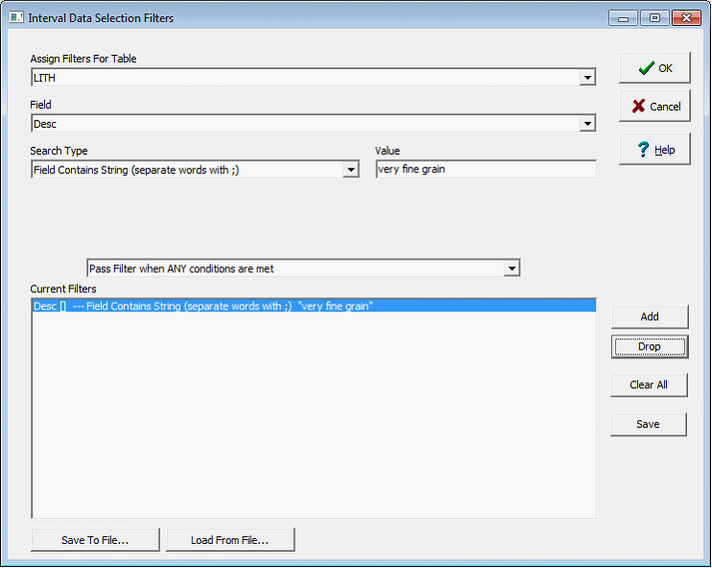
The Interval Data Selection filters can be divided into two parts. The upper half of the screen builds and modifies filters, while the lower half shows the active filters and the pass relationship between different filters. To create a new filter, select the table and field for the filter from appropriate dropdown menus. The example below filters intervals in the LITH table by data in the DESC data field. Next, select the filters Search Type. With one exception (Interval Thickness In Range) the search type tells Petra what the filter should look for inside a field:
Not Equal to Value Equal to NULL Not Equal to NULL Value in Range Field Contains String
Interval Thickness in Range eliminates intervals that are thicker or thinner than a given range. Finally, select the Add button to add the filter to the Current Filters list at the bottom of the box. In the example below, the filter is set to include only intervals that contain the words, very fine grain
Up to 10 filters can be active at once. There are two options for how to combine multiple filters: Pass Filter when ANY conditions are met and Pass Filter when ALL conditions are met. The choice of these two options can have a significant influence on which intervals are plotted on the cross-section. For more on combining multiple filters, see Appendix 2. Pass Filter when ANY conditions are met this will pass any interval where at least one of the conditions is met. This is the more permissive option, since only one of the filter criteria needs to be met to pass. Pass Filter when ALL conditions are met this will pass any interval only when all conditions are met. This is the more restrictive option, since all filter criteria need to be met to pass.
Plotting Interval Data in the Cross Section ModuleThe Cross Section Module can display any combination of interval data colors, patterns, markers and text. To display interval data for a well in the Cross Section Module, select Wells>Plot Interval Data. This box shows a list of the interval data tables on the left along with a series of tabs on the right that control how interval data (Style, Text, Filters) are shown. First, select the interval data table or tables to display. Petra can show multiple intervals at the same time, though its generally better to keep different interval tables in different tracks. In the example below, only the LITH table is selected. The Style tabThe Style tab governs how the interval data is displayed on the Cross Section.
Use Interval Fill Color This option tells Petra to fill the interval with the intervals color. Use Interval Fill Pattern - This option tells Petra to fill the interval with the intervals pattern. Use Interval Marker Symbols - This option tells Petra to fill the interval with the intervals marker symbols. The Marker Scale factor below changes the size of these symbols. The individual intervals marker fill can also be overridden with the Marker Fill Mode below. Text Positioning Text can be positioned at the top, middle, or bottom of an interval. Select the dropdown by default labeled Text At Top of Depth Interval to change where text is plotted. Combining Text Horizontally or Vertically This changes how multiple text fields are displayed. Combine Text Horizontally lists additional text fields to the right of the first text box. Combine Text Vertically stacks additional text fields on the bottom of the first text field. Separate Text with Space This option changes how different fields are separated when plotted horizontally. Horizontally combined text boxes can either be separated with a space, slash, a dash, or a comma. Text Label Size This option sets the size of text (in inches). Keeping this option at 0 is a good default. Remember that an absolute text size probably wont be appropriate for both computer screens and large paper plots; 1 inch letters will look huge on a computer screen, but will be normally sized on a large wall plot. Marker Scale Factor This option sets the scale of the interval markers. Setting the scale factor to 0.5, for example, plots all markers at ½ their original size. Marker Fill Mode Though every interval stores information on how to display markers, this option overrides the fill mode for all displayed markers on the cross section. Note that this does not change the settings stored in the interval. Pattern Scale Factor This option sets the pattern scale, or density, of the lithologic pattern fill. Higher numbers here generate higher pattern density. The Text tabThe Text tab sets the specific data fields to be displayed as text.
To add text, select the appropriate table on the Interval Data to Plot dropdown menu and a data field from the Data Fields to be Posted By Intervals dropdown menu on the right. Select the
The Filters tabFilters provide more control over which intervals are displayed on the Cross Section Module. Intervals that do not meet the filter criteria are not displayed. To create or modify a set of filters, select the Set Filters button on the Filters tab. For more information on filters see the Using Filters section of this document.
Interval Data in the Map ModuleThe Map Module can show and grid interval data on deviated and horizontal wells. Petra can show a rectangular area with the intervals pattern and color along the wellbore, each intervals marker symbol, or both. Intervals are a good way of showing the encountered lithology, or for quickly showing the wellbores footage spent in, above, or below a target stratigraphic unit. Gridding with Interval dataDeviated and horizontal wells can generate data spread along the wellbores path. Interval data is a good way of displaying and incorporating multiple data points along a wellpath into a grid. Petra can grid any numerical interval field designated as a real value. Date and text interval fields cant be used in gridding. In the Map Module select Contours>Create Grid from the menu bar at the top of the screen. Here, select the relevant data, grid size, and surface style; Petra can integrate interval data into a grid using zone data, tops, overlay contour lines, or other XYZ data. On the Interval Data tab, select the Active option to use the selected interval table and numerical interval field in gridding.
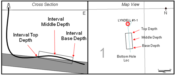
Note that there are a couple of ways to modify which intervals are used in gridding: intervals can be pared down by quality codes, zones, or interval filters. The Skip Well if Quality Code Contains option allows the user to skip wells that have specified quality codes. Here, enter one or more values separated by a semicolon to indicate intervals that are NOT to be used for gridding. Intervals must Fall within Depths of Zone - This option limits which intervals are used in gridding to only the intervals inside the specified zone definitions. The WELL zone covers all depths, and consequently all intervals. Be careful when using zones and horizontal wells. Note that this zone criteria works uses the zone interval definitions, which are often defined by tops. Horizontal wells that stay entirely within a zone and never reach the base will not have a base top picked, and will consequently be excluded from gridding. Apply Interval data Filters - This option provides more direct control over which over which intervals are used in gridding. Intervals that do not meet the filter criteria are not gridded. To create or modify a set of filters, select the Set Filters button on the Filters tab.. For more information on filters see the Using Filters section of this document. Use Interval Top/Middle/Base Depth - This option sets where numerical real value interval fields are contoured. Especially with longer intervals in horizontal wells, this difference can significantly change where a data point is plotted. Note that this option is grayed out when gridding interval tops and bases. In the example below, a single interval in the wellbore is outlined in with a box on the cross section on the left. While the top and base of the interval have a specific XY location on the map, other data (such as an average porosity value) can grid that value at the XY position at top of the interval, at the middle of the interval, and at the base of the interval.
Apply Subsea TVD Correction to Interval Field Value - This option instead corrects to SSTVD by subtracting the KB elevation. By default, Petra uses the surveys TVD when contouring the top and base of intervals. This option is essential when incorporating interval data into SS structure maps. XYZ File Containing Int Data Used in Gridding - This option creates a text file containing the X and Y coordinates (using the projects map projection) along with the interval value used in gridding. Specifically, Petra creates a *.XYZ file in the projects GRIDS folder. This file will be named after output grid file name with a _INTDATA.XYZ suffix.
Plotting Interval ColorsInterval colors are plotted in a filled rectangle along the wellpath. This is useful for aerially representing continuous information in a wellbore, such as changes in lithology, biostratigraphic assemblages, or even gas shows. In the Map Module, select Options>Interval Data on Well Path Select the appropriate interval table to display from the dropdown, and select the Plot Filled Rectangle option under the Interval Indicator dropdown. With this option, Petra fills the rectangle with each intervals color.
Filters provide more control over which intervals are displayed on the Map Module. Intervals that do not meet the filter criteria are not displayed. To create or modify a set of filters, select the Set Filters button on the Filters tab.. For more information on filters see the Using Filters section of this document.
Plotting Interval Data MarkersInterval markers are along the wellpath at the top, middle, or base of the interval. Unlike the filled rectangle, interval markers can be plotted at a user-defined orientation. Interval markers are useful for representing discrete markers, such as fractures or MWD tool changes.
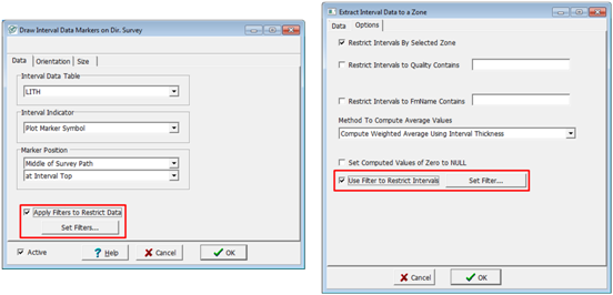
In the Map Module, select Options>Interval Data on Well Path Select the appropriate interval table to display from the dropdown, and select the Plot Marker Symbol option under the Interval Indicator dropdown. Next, select the position of each intervals marker relative to the wellbore (middle, left, or right of the wellbore) and the position of the marker along the interval (top, base, midpoint). Note that filters can also be applied to the interval data; only intervals meeting the filter criteria are shown. In the example below, the Fractures interval table stores a horizontal line marker for every interval.
To set the direction of each marker, select the Orientation tab. Markers can be perpendicular to the borehole, parallel to the borehole, or have a user-defined orientation, or azimuth. This user-defined azimuth can either be a constant azimuth for all interval markers in all wells, set for all intervals markers for each well by a zone data item, or for each individual interval in each well by an interval data field. When storing individual fractures in a wellbore, storing azimuth data in each interval captures the most information and allows for each marker to have its own orientation. In the example below, the AZI data field gives the compass azimuth for each fracture.
To set the size of each marker, select the Size tab. The size of each marker can either be a constant for all interval markers in all wells, set for each well by a zone, or for each individual interval in each well by an interval data field. Note that the marker size can either be set to use map XY units, feet, or meters. Selecting a constant size of 0 sets a default marker size, as shown in the example below. The Marker Scale Factor can scale the size of a zone- or interval field-defined marker by anything between 0 and 100.
Storing Interval Data to a ZoneIts sometimes useful to extract data from intervals to a zone. Zones are easily used in calculations and mapping. In the Main Module, select Compute>From Interval Data>Extract Interval Data To Zone Under the Extract Interval Data from dropdown menus, select the appropriate interval table and field. In the example below, the RW from SP interval data is selected from the Petrophysics table. Petra can either extract the interval field data or the interval thicknesses. In the example below Petra will calculate an average of the RW from SP interval data. Since a single zone can contain multiple or overlapping intervals, there are a few different ways to extract this field or interval thickness data:
First/Last value Min/Max of values Average of values (weighted or unweighted by thickness on the Options tab) Sum of values Count of values Sum of interval thicknesses Average of Thicknesses Count of intervals
Next, select the zone and data item where the interval data will be stored. Note that this tool uses the selected zones definitions (where fm tops or depths define the top and base of the zone) to limit the extraction only to intervals intersecting the zone. A default zone definition of -99999 to 99999 will include every interval in the wellbore. Next, select when the field value should be stored to the zone data item. Petra can store the interval data meets the following criteria: When the item is present This option stores the interval field value to the zone data item when the interval data contains a value. This is useful for most applications, such as storing a petrophysical value to a zone. Item is absent This option stores the value when the interval data field is null. Practically, this option is only useful when extracting the sum/average of interval thicknesses or interval counts. As an example, extracting a count of intervals when the porosity interval data is absent generates a well-by-well count of intervals missing porosity values. Range This option stores the interval field value when the field value falls between a minimum and maximum value. Contains text This option stores the interval field data when the interval field contains specified text. Matches text - This option stores the interval field data when the interval field exactly matches the specified text.
The Options tab contains further options for limiting the intervals used in the extraction.
Restrict Intervals By Selected Zone - By default, Petra only uses intervals that intersect the selected zones definitions (where fm tops or depths define the top and base of the zone). Note that undefined zones extend from -99999 to 99999 MD, which includes every interval in the wellbore. Deselecting this option will not limit intervals by zone definitions. Alternatively, intervals can also be limited by interval quality codes or FmName fields. Method To Compute Average Values - When computing an average value for the interval, Petra normally uses weighted averages, where thicker intervals contribute more to the average than thin intervals. Selecting Compute UnWeighted Average gives equal weight to all values regardless of interval thickness. Set Computed values of zero to null - Remember that a null is not equal to zero. Mistaking the two can generate spurious maps and calculations. The option sets extracted values of zero to a null value. Use Filters To Restrict Intervals - Filters provide more control over which intervals are used in the zone extraction. Intervals that do not meet the filter criteria do not contribute to a zone data item. To create or modify a set of filters, select the Set Filters button on the Filters tab. For more information on filters see the Using Filters section of this document.
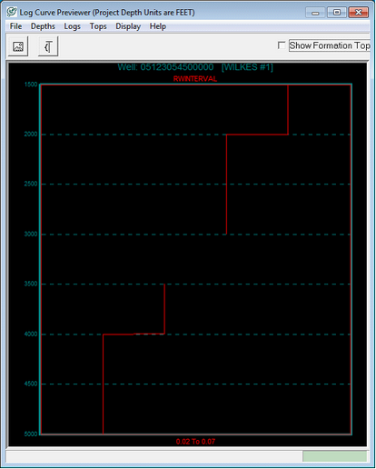
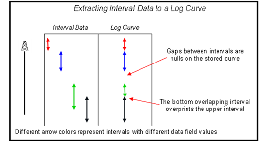
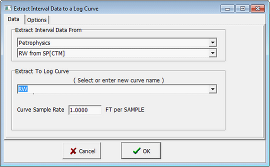
Storing Interval Data to a Log CurveIts sometimes useful to extract numerical data from intervals to a log curve. Logs curves are easily displayed on cross sections and can be used in petrophysical calculations to create new composite curves. In the Main Module, select Compute>From Interval Data>Extract Interval Data To Curve Under the Extract Interval Data from dropdown menus, select the appropriate interval table and field. In the example below, the RW from SP interval data is selected from the Petrophysics table. Petra extracts an interval field data value and applies it to that intervals corresponding footage on a log curve. As an example, an interval from 1500 to 2000 with a RW of 0.06 will translate into a log curve with a repeating RW of 0.06 from 1500 to 2000, as shown in the example below.
Intervals often have gaps and overlaps between intervals. Gaps between intervals are simply stored as null values on the curve. Where log intervals overlap, the bottom interval overprints the upper interval. To resolve these gaps and overlaps in the data, see Resolving Gaps and Overlaps in this document.
Under the Extract Interval Data from dropdown menus, select the appropriate interval table and field. Next, select the name of the log curve. In the example below, the RW from SP from the Petrophysics table will be stored as a new RW curve. These curves can be stored at any sample rate, though 1 foot- and ½ foot-spacing are the most common.
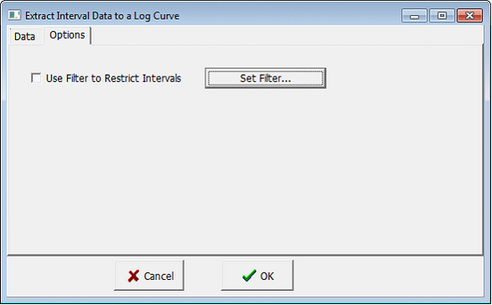
The Options tab contains further options for limiting the intervals used in the extraction. Filters provide more control over which intervals are used in the zone extraction. Intervals that do not meet the filter criteria do not contribute to the log curve. To create or modify a set of filters, select the Set Filters button on the Options tab. For more information on filters see the Using Filters section of this document.
Storing Log Curve Statistics to an IntervalIts sometimes useful to extract numerical data from log curves to an interval. More specifically, this tool calculates statistics over a selected log curve between the top and base of each interval and stores the result as a interval data field. This statistical measurement is stored to a data field in a selected interval table. When stored as interval data, log curve statistics can be easily used in petrophysical calculations or compared with other interval data fields. In the Main Module, select Compute>From Logs>Extract Log Stats to Int Data First, select the desired log curve from the dropdown menu at the top of the screen. In the example below, the GR curve is selected. Note that this tool will calculate log statistics on aliased curves, as well. Next, select the desired interval table from the Interval Data table on the lower left side of the screen. In the example below, the LITH table is selected, so the statistics measured will be stored in interval data fields in the LITH table Finally, select the desired statistics and the desired location. In the example below, a mean (or average) will be calculated for the GR log. The calculated average will be stored in a interval data field called GammaStat. Petra stores statistics out to 7 decimal places, even though the interval data field may only show fewer trailing decimals.
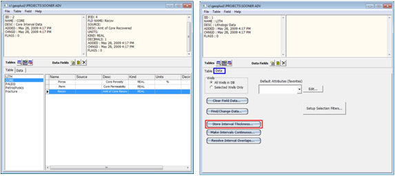
Storing Interval Thickness to an Interval FieldThis operation stores each intervals thickness to a specified field in that interval. Select the Maintenance button on the bottom of the Interval tab on the Main Module. On the table tab, select the interval field that will store the interval thickness. In the example below on the left, the Recov field on the CORE table is selected. Next, under the Data tab (highlighted in blue on the example to the right) select Store Interval Thickness (highlighted in red).
The example below shows that the sidewall core thicknesses (in this case given a thicker interval) all store thicknesses of 2 feet in the Recov field.
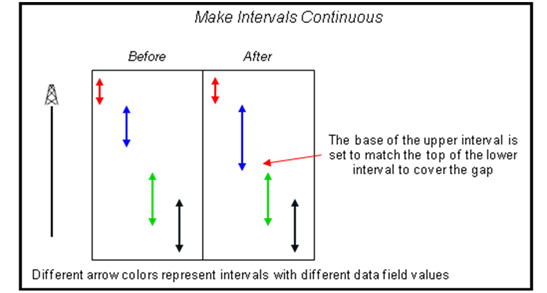
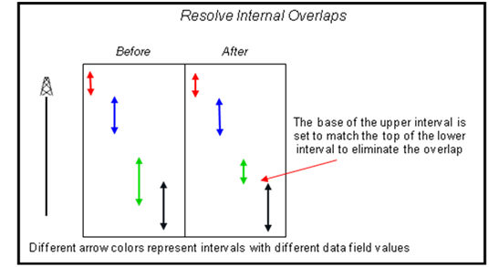
Gaps, Overlapping Interval Data, and Bulk ShiftsInterval data is often at the wrong depths, or contains overlapping intervals or gaps. Though interval data is designed precisely to handle this incomplete and contradictory data, its often useful to convert interval data into one continuous chain for display or calculations. Interval data can also become out of sync with other well data; moving interval data up or down with a bulk shift easily remedies the discrepancy. To perform these operations on a single well, select the Edit Details button on the upper right corner of the Interval tab on the Main Module. Next, Edit dropdown on the menu bar at the top of the window, select Make Intervals Continuous button or Resolve Internal Overlaps, or Bulk Shift. Make Intervals ContinuousThis option eliminates overlaps where two different intervals cover the same footage. With this option, Petra moves the base of the upper interval to match the top of the lower interval, as shown in the example below.
Resolve Internal OverlapsThis option eliminates gaps between intervals. With this option, Petra moves the base of the upper interval to match the top of the lower interval to cover the gap, as shown in the example below.
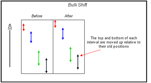
Bulk ShiftThis option adds or subtracts a specific number to all interval depths. A negative number moves all intervals up, while a positive number moves all intervals down.
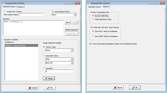
Calculations with Interval DataPetra can perform basic calculations on interval data columns, zone data items, or constants. This operation is performed on all intervals in selected interval table in either the current well or for all wells selected in the Main Module. To calculate a new interval data column from another, select the appropriate interval table on the appropriate well, then select the Calculate Column on the Interval tab First, establish where the output will be stored. Petra can store data to a new or preexisting column in the selected data table. To store data to a new column, select Create New Column and enter in the new columns name. To use a column thats already in the data table, select Use Existing Column, and select the column from the underlying dropdown menu. Be careful when using an existing column, as this operation can overwrite any data already entered. Next, enter an equation using variables and mathematical operators. For a list of available operators and sample equations, see appendix 3. The variable on the left side of the equal sign is the result variable. Note that the variables here are just text and will be assigned later, so they can be either specific (porosity) or general (A). Note that equations can be saved and loaded again at a later date with the Save and Load buttons on the right side of the screen. In the example below, porosity data is being used to calculate a permeability value. Now that the equation is entered, select Assign Vars. This populates the Variable List in the bottom left corner of the window with the variables written in the equation. Select a variable from the Variable List, and select a column, zone data item, or constant from the relevant dropdown menus on the right. Select the Assign button. This will change the entry in the Variable List box to reflect the correct variable. The Options tab has a few more controls over the calculation. The calculation can be performed on only the currently selected well in the Main Module, or on all wells selected in the main module. Petra stores a null value whenever theres a missing variable in the calculation, but the Save ZERO value to Database can overwrite this null value with a zero. By default, Petra overwrites all interval data fields during the calculation. Deselecting the Overwrite Existing Database Values with Calculation Result forces Petra to leave existing database numbers alone, limiting the calculation to only filling in null values. To perform the calculation, select the OK button.
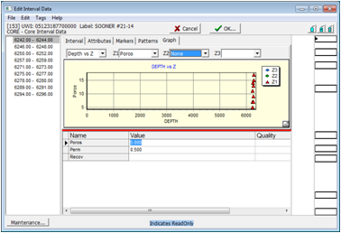
Graphing Interval DataPetra can plot any numerical interval real value versus depth or another real value. This can be particularly useful for quickly seeing how a quantity such as mud weight changes with depth, or understanding the relationship between two different kinds of data like porosity and permeability. To view an interval graph, first select the correct well in the Main Module. On the Interval tab, select the right interval table. In the example below, the CORE table is selected. Finally, select the Edit details button in the upper right on the Interval tab.
On the Graph tab, select Depth vs Z or X vs Z on the first dropdown menu. Depth vs Z shows the selected values for the interval fields selected on the Z1, Z2, and Z3 dropdown menus on the vertical axis relative to depth on the horizontal axis. The example below shows how porosity varies with depth.
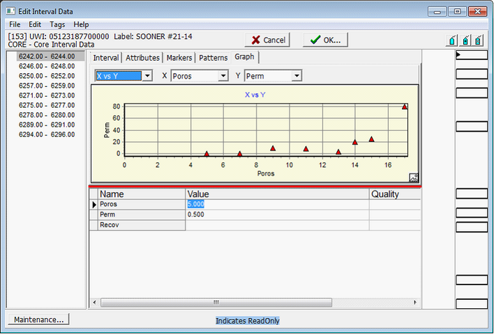
X vs Y shows a scatter plot for the two interval fields selected on the X and Y dropdown menus. The X value is plotted on the horizontal axis, and the Y value is plotted on the vertical axis. The example below shows how permeability varies with porosity
APPENDIX 1: Setting Default tables and FieldsChanging these default interval tables can be useful from an administrative perspective. Changing these tables ensures that all new projects will be created with the same interval tables and fields, though these can always be changed inside Petra. When creating a new project, Petra looks at a file called INTDATA.DEF located in the programs Parms directory. On most standalone installations, this will be located in C:\geoplus1\Parms. This file contains the default tables and fields that will be created in a new project. Its important to not edit the default interval table file (INTDATA.DEF). Instead, copy the INTDATA.DEF file to a new file called INTDATA.USR. Make all new changes to the new file called INTDATA.USR. Petra first looks for INTDATA.USR before it looks for INTDATA.DEF. The default version of this file contains three tables: LITH, CORE, and PALEO.
Table: LITH - Lithology Field: Desc - Description
Table: CORE - Core Interval Data Field: Poros - Core Porosity Field: Perm - Core Permeability Field: Recov - Amt of Core Recovered
Table: PALEO - Paleo Data Field: FmName - Formation Name Field: Bug - Fossil Name Field: Age - Age of Zone
Petra reads the INTDATA file and builds interval data based on comma-delimitated values.
TABLE, TABLE NAME, Table Description FIELD, KIND, NAME, SRC, Field Description, UNITS, DECIMALS
TABLE This signifies that the entry is for a new table. Table Name This is the name of the table. Its a good idea to separate tables based on genetically related data, such as mudlogs, core descriptions. Remember that tables, unlike zones, are completely independent of stratigraphy, so it is probably easier to lump all related data together rather than break out intervals based on specific formations. Table Description - This sets a brief description of the table. In the example, the LITH fields description is Lithology Data. Remember to put quotation marks around the description. FIELD This just signifies that the entry is for a new field. Make sure all new field entries are prefaced by FIELD. Kind Fields can store three kinds of data: Real Values, Date Values, or String Values. The letter here tells Petra what kind of data this field will store R for Real values, D for Date values, and S for String values. Real values simply store numbers, such as porosity or permeability. Dates store calendar days as MM/DD/YYYY. String values store text, like core descriptions. Name This is the name of the field. SRC This sets the user source for the specific field. User sources are useful for distinguishing between different users interval data in a multiuser environment. Field Description This sets a brief description of the field. In the example, the Recov fields description is amt of core recovered. Remember to put quotation marks around the description. UNITS This sets the units of the field. DECIMALS This sets the number of decimals shown for real value (numerical) data. Though its a good idea to set this value to 0 for string and date fields, its not necessary APPENDIX 2: ANY and ALL with multiple Interval Data FiltersThere are two options when combining multiple filter combinations. Data can either pass ALL conditions, or ANY of the conditions. The difference between the two is significant, and is best illustrated by an example with two data filters:
Object is yellow Object is smaller than a breadbox
Well apply those filters to three objects: a Banana, an Apple, and a Schoolbus. When ALL conditions need to be met, only the banana passes the filter because it is both yellow and smaller than a breadbox. When the filter just requires ANY condition to be met, each object only needs to pass one of the filters. In this example, all three objects pass the filter. The apple is smaller than a breadbox, the schoolbus is yellow, and the banana is both smaller than a breadbox and yellow.
APPENDIX 3: Equations and Mathematical OperatorsPetra recognizes a wide variety of mathematical operators:
+ Addition - Subtraction * Multiplication / Division ** Exponent ABS(x) - Absolute value of x ACOS(x) - Arccosine of x (in radians) ASIN(x) - Arcsine of x (in radians) ATAN(x) - Arctangent of x ( in radians) COS(x) - Cosine of x in radians COSH(x) - Hyperbolic cosine of x (radians) EXP(x) - e to power of x INT(x) - Truncated value of x LOG(x),LN(x) - Natural Log of x LOG10(x) - Log based 10 of x MAX(x,y) - Maximum of x and y MIN(x,y) - Minimum of x and y ROUND(x) - Rounded value of x SIN(x) - Sine of x in radians SQRT(x) - Square root of x SQR(x) - x squared SINH(x) - Hyperbolic sine of x (radians) TAN(x) - Tangent of x in radians TANH(x) - Hyperbolic tangent of x (radians)
Operators are performed in the following precedence: 1 Exponent 2 Multiplication and division 3 Addition and subtraction
Use of parentheses can change the order of precedence.
Example Equations: GRN=GR - MEAN_GR + MEAN LOGNRM = LONORM+(LOG-PICKLO)*(HINORM-LONORM)/(PICKHI-PICKLO) LOGNRM = LOG+ LOGPICK - GOODPICK SW = ( RW/(RT * (PHI**M)))**(1/N) R = ((A+B*(C-1.0))/100 R = X*SIN(A)+Y*COS(B) R = LOG10(X) R = X*X or R = SQR(X) R = X**Y (x raised to the y power)
|
 - This option adds a new interval data table. Selecting this option brings up a dialogue box to add the new tables name and description. A newly created table contains no new fields.
 - This option edits just the name and description of an existing interval data table. To edit the fields inside the interval, select the Data Fields option on the Maintenance screen.
 - This option deletes the entire interval data table, along with all the fields and data contained within the table.
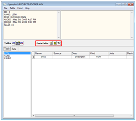
 - This option adds a new interval field to the selected interval data table. Selecting this option brings up a dialogue box to add the new fields name, description, and attributes. The Kind dropdown box sets the kind of data the interval field stores: a Real Field, Date Field, or String Field. Real Fields simply store numbers, such as porosity or permeability. Dates store calendar days as MM/DD/YYYY. String values store text like core descriptions. For Real fields, the Units box sets the displayed units of measurement, while the Decimal Places for Display option sets the displayed trailing decimals.
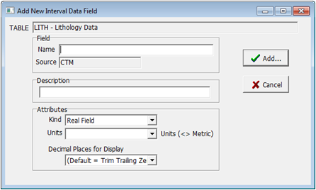
 - This option modifies the name, description and attributes of the selected field.
 - This option deletes the selected field.
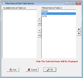
 button.
 button on the Defaults section on the Attributes tab (highlighted below). This stores the current scheme of colors and patterns as a default attribute so it can be used later on different intervals.
 or hold down the CTRL key. Next, select the desired intervals on the graphical representation of the intervals on the right side of the screen. Note that the selected or tagged intervals have a small black triangle on the far right (highlighted in the example below). In the example below, all the very fine grained sandstones have been tagged.
 button. To drop all tags, select the
  button.
 button on the Defaults section of the Attribute tab. This applies the current Default scheme of colors, markers, and patterns to all tagged intervals.
  button only applies the default scheme to the currently selected interval, while the
  button applies the default scheme to all intervals in the well.
 button on the Defaults section on the Attributes tab. In the example below, there are three default schemes based on lithology: the blue interbedded siltstone/sandstone, the pale yellow very fine grained sandstone, and the bright yellow fine grained sandstone.
 button. In the example below, red stars have been added for all intervals with porosity above 10%, and a black X for all intervals with porosity below 10%.

 button to adds the field to the list. Items at the top of the list will be at the top (for vertically combined text) or on the left (for horizontally combined text). Selecting the Include Text Labels option adds the field name as a prefix before each data field. Particularly elaborate displays can also be saved as a template in a *.IDF file with the Save/Load Template buttons.