Advanced tab

Click Here for a "How-To" guide on creating Contour Grids

The Advanced tab changes settings on how Petra creates grids.  While a couple of these settings actually modify how Petra uses missing or poor quality data (Substitute Zero for Missing SS Datums, and Skip Well if Quality Code Includes), most of the settings govern the specific settings of the gridding algorithms.

It’s generally quicker to focus time and effort on drawing a few contour lines to add interpretation rather than using these settings.  Remember, it’s not necessary to draw a complete set of contour lines in order to greatly enhance the gridding process.  Even just a few key contour lines can have an enormous (and quick) effect on the computer-generated grid.

The “Defaults” button on the lower right corner of this tab reverts all settings back to the default settings.  The default settings are a good all-around choice for most gridding.

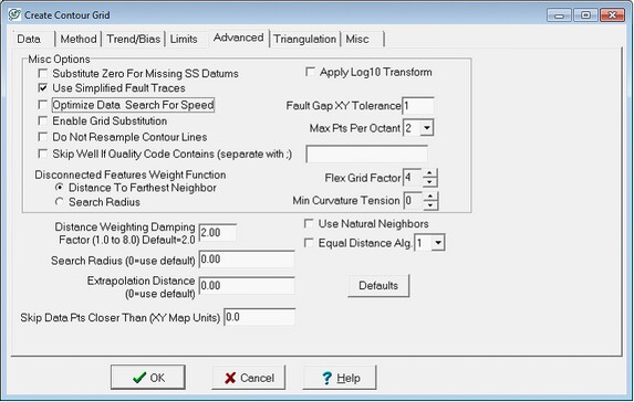
The Create Contour Grid Advanced tab

Misc Options

"Substitute Zero For Missing SS Datums" – Plotting maps in subsea (or “SS”) attempts to eliminate the effect of surface topography on subsurface structures.  Instead of plotting subsurface features according to their measured depth (MD), SS depths are referenced to sea level at 0’ elevation; depths below sea level are in negative numbers and depths above sea level are positive.  The equation to calculate a fm top’s SS is straightforward: Elevation – MD = SS.  Elevation is usually provided as ground level (GR), kelly bushing (KB), or derrick floor (DF).

In the example below, the reservoir in the subsurface is perfectly flat.  There’s a significant change in elevation across the area (blue arrows), however, which has a large effect on the overall measured depth (black arrows) to the reservoir.  The best way to illustrate the true nature of the reservoir’s structure is with SS depths (red arrows), which are exactly the same for all wells.  The third well, however, is missing an elevation datum, so accurately calculating its SS depth is impossible.  Normally, when the reference datum is missing, Petra simply leaves the SS depth null.  These null values have no effect on gridding SS surfaces.  

Selecting the “Substitute Zero For Missing SS Datums” option, however, will substitute in a zero for the missing elevation.  For areas of uniformly low elevation this is a reasonable assumption.  For areas with changing elevation, however, this can grossly distort the map.  In the example below on the right, a zero elevation substitution ignores the effect of elevation, which causes a large (and entirely fake) syncline underneath the well missing a elevation datum.

Use Simplified Fault Traces – This option simplifies the number of points on drawn fault lines in order to accelerate gridding. Fault lines on the overlay – particularly those drawn using the “stream” mode - can contain a large number of redundant points.  Since faulted grids require triangulation of each fault line node, simplifying the fault can greatly accelerate gridding time and reduce overall grid file size.  This option does not change the fault line as drawn on the overlay.

Optimize Data Search For Speed – This option presorts data points by location in order to accelerate gridding.  This clustered data, however, tends to generate radial grid artifacts.  Most modern computers are fast enough to not need this option.

Enable Grid Substitution - Use this option to use values from another grid file to fill in sparse control point areas.  This unlocks the Grid Subst tab.  Here, select an existing grid in the default grid directory.  Petra will substitute values from this grid wherever there are missing values on the new grid.

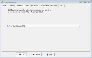
The Create Contour Grid Grid Substitution tab

Do Not Resample Contour Lines – In order to use a drawn contour line, Petra needs to resample the line into a set of discrete points.  By default, Petra calculates an optimum sample based on the specific grid’s spacing.  This option instead forces Petra to use all available data points from the contour line, which can greatly oversample the data and generate erroneous ties to the contour line.

Skip Well if Quality Code Contains – This option skips data points from wells that have specified quality codes.  Here, enter one or more values separated by a semicolon to indicate wells that are NOT to be used for gridding.

Disconnected Features Weight Option – The Disconnected Features surface style depends on “weighted averages”, in which nearby data points contribute more to an individual grid point’s average than distant data points.  This option changes how the Disconnected Features surface style averages different data points.

The weighting of different data points is determined by a ratio between the distance of a data point to the grid node and a “total distance.”  This option simply sets how Petra defines this “total distance.”  Distance to Farthest Neighbor uses the distance to the furthest well used in the octant search, while the Search Radius option instead uses the entire search radius (which by default is half the diagonal of the gridded area).  Effectively, the nearest neighbor distance creates a localized weighting relationship for every grid node, while the search radius setting uses the same weighting relationship for every grid node.

Apply Log10 Transform – Highly variable data such as production information can generate anomalously broad contours during normal gridding.  This option applies a transform to the data to “tighten” contour lines around highly variable data.  The output grid will have the original Z value units.

Mathematically, the Log10 transform has three steps.  First, the filter applies a Log10 transform to all data points.  In the example below, the six wells with values of 10 surround one well with a value of 1000 shown on figure A.  Taking the LOG10 of these data points changes them to six wells with a value of 1 surrounding a single well with a value of 3 (Log10(10) = 1, Log10(100) = 3).  Gridding these transformed values generates a simple grid with values between 1 and 3 as shown on figure B. Finally, Petra converts the data points and the new grid back to their original data points with the inverse of Log10, 10^X.  Effectively, this changes the original linear slope between the central, large data point and the outlying smaller data points from a linear relationship to a power relationship.

Practically, the transformed grid reduces the regional effect of the large value in the center.  Generally, adding the LOG10 transformation will generate a more conservative grid with highly variable data than a simple linear surface style alone.

Fault Gap XY Tolerance – Faulted grids sometimes have small white triangles on color-filled grids near fault node points.  Changing this option changes how Petra constructs a faulted grid, which can eliminate these artifacts.  The default value is 1.0 XY unit, and should be kept between 0.5 and 3.0. A value that is too large may cause other unwanted white space between grid cells

On rectangular grids, Petra handles faults by creating a triangular grid inside the regular rectangular network of grid nodes.  Where the overlay fault crosses a set of four grid nodes (as in the example below), Petra adds more data points a small distance away from the drawn overlay fault line on the normal rectangular grid spacing.  Petra then constructs a triangular grid using these new points to break the grid across the fault.  This “Fault Spacing” option sets the maximum distance between the drawn fault and the newly created points.

Fault Gap Tolerance

Max Pts Per Octant – Petra interpolates the value of each grid node from surrounding data points.  This option sets the maximum number of data points in each octant used for each grid node, and can be anywhere from 1 to 8.  For example, with a value of 2 the gridding process will use a maximum of 16 data points (2 for each octant) distributed around the grid node.

When determining which data points will be used for each grid node, Petra first divides the area around the grid node into eight wedges, or “octants.”  Petra then uses the closest data points (up to the maximum set by this option) in each octant for calculating an individual grid node’s value.  Dividing the surrounding data into octants helps avoid grid nodes that are too heavily biased by data points in one direction.

Max points per octant set to 1 (left) and 2 (right)

Flex Grid Factor – This option changes the relative strength of the “Smooth Contours using Grid Flexing” option.  Low Grid Flex Factor create final grids that  look like the original surface style, while higher Grid Flex Factors will create a grid that looks more like a Minimum Curvature grid.

When the “Smooth Contours using Grid Flexing” option is selected (on the Method tab), Petra first interpolates the data points with the selected surface style, then adds an additional step to interpolate both the original data points and the newly created grid values with the minimum curvature gridding algorithm.

Mathematically, this option controls the decimation of the initial grid, and can be set from 2 to 12.  When this option is set to 2, every other original grid point will be used in the Minimum Curvature step.  In this case, a large number of initial grid points remain which constrains much further interpolation from the second minimum curvature interpolation.  When this option is set to 12, only every 12th original grid point will remain.  The relative low number of initial grid points allows for more interpolation from the Minimum Curvature step.  In short, the lower the Grid Flex Factor, the more the final grid will look like the original surface style.  Higher Grid Flex Factors will create a grid that looks more like a Minimum Curvature grid.

Min Curvature Tension – This option sets the flexibility, or “tension”, of the Minimum Curvature surface style and the Grid Flexing option available on the Method tab.  This value can be set between 0 and 9.  A grid with a low tension setting easily folds and bends to accommodate changes in the data, while grids with a higher tension folds less easily.  Practically, high tension grids – particularly above 5 - have smoother and more even contours but may not honor the original data as well as lower tension grids.

Specific Surface Style Options

Distance Weighting Damping Factor – Both the Sample Weighing With Slopes and Sample Weighing Without Slopes surface styles depend on “weighted averages”, in which nearby data points contribute more to an individual grid point’s average than distant data points.  This parameter determines the relative contribution of close data points versus more distant data points to the final data grid value.  Petra can use any value from 1 to 8, with a recommended default setting of 2.  With a small factor, more distant data points have more influence on an individual data point which tends to average the grid node; this usually results in a smoother grid.  With a larger factor, close data points influence the individual grid much more than more distant data points.  The recommended value for this factor is 2.

Mathematically, when either of the sample weighing surface styles calculates an individual grid node, Petra uses the adjacent data points and multiplies them by an inverse of the distance to the grid node (1/Dn).  Multiplying by the inverse of the distance minimizes the contribution of more distant datapoints (with a larger D) relative to more proximal ones (with a smaller D).  The Distance Weighing Damping Factor, n, is the power of the distance in the inverse, which magnifies or minimizes the inverse’s effect on distant data points.

The example below walks through a single grid node (the + in the center) calculated from three surrounding points.  The map view on the left shows that two data points have values of 15 and are 10 units away from the grid node, while one data point has a value of 10 and is 3 units away from the grid node.  The formula for the calculating the grid node is below the map view.  Filling in the values on the left side of the figure, it is a little easier to see how the Distance Weighting Damping Factor, n, affects the formula.  Larger values of n decrease the relative contribution of the more distant wells with a value of 15, which drops the averaged grid node value.

Using a  damping factor to prioritize close data points at the expense of more distant data points

Search Radius – To calculate a single grid node, Petra interpolates values from surrounding data points.  Most rectangular gridding uses an “octant” search, where Petra uses only the nearest data points (set by the “Max Pts Per Octant” setting) from each of the eight pie-shaped wedges, or “octants.”  This option sets the radius of this search in XY units.  The default, set with a zero value, is a fairly large search radius of half the diagonal of the gridded area.

A small search radius only uses close data points (left) while a larger search radius can use use more points (right)

Dividing the surrounding data into octants helps avoid grid nodes that are too heavily biased by data points in one direction.  If the specified search limit is too small, the grid may contain null values in areas of sparse data control.

Extrapolation Distance - This option sets the distance (in XY units) to extrapolate the grid beyond the data points. The default value of 0.0 extrapolates the grid two grid cells beyond the actual data points or up to the data limits set by the "Grid Extrapolation" option selected in the Limits section.

The extrapolation distance will only extend the grid in multiples of the grid spacing.  The “convex hull” blanking method (on the Limits tab) also automatically nulls any grids beyond a polygon defined by the outer-most data points, which can negate any changes made to the extrapolation distance.

Skip Data Pts Closer than (XY Map Units) – Close data points can cause unwanted gridding artifacts.  When Petra finds two data points that are within this setting’s value of XY units together, it only uses the first one it finds.  As an example, setting this value to 100 will skip any other data points within 100 XY map units.  For well data, Petra will use the well with the lower WSN.

Use Natural Neighbors – This option causes most surface styles to use a “natural neighbors” triangulation search instead of the normal octant search when selecting data points to interpolate for each grid node. This tends to provide a more localized interpolation, which can benefit grids with dense data point coverage.  Since this adds an additional pre-gridding triangulation stop, this option can increase gridding time.

When deciding which data points to use for each grid node, most rectangular grids styles (Highly Connected Features, Disconnected features, Simple Weighting With/Without Slopes) use an octant search where the area around a grid node is divided into eight wedges, or “octants.”  This octant search ensures that data points used for the grid point interpolation are evenly geographically distributed.  A natural neighbors search, in contrast, selects surrounding data points that can be connected by a triangular network. This option just changes how Petra selects the data points for interpolation, so the output will be a normal rectangular grid.

Octant search selects data points in 8 wedges around the node, while a natural neighbors search uses a triangular grid

Equal Distance Alg. - This option adds additional triangulated data points in between widely spaced data points before normal gridding.  This helps to fill in areas of sparse data coverage to better preserve regional trends on the grid.

Mathematically, this step performs a simple triangulation between distant data points and adds them to the grid before performing the normal gridding with the selected surface style.  These triangulated data points can have a refinement of 1, 2, or 3, as set by the adjacent drop down menu (for more information on refinement, see the “Triangle Refinement” in the Triangulation Help document).  These additional data points are used along with the original data points during the normal gridding.  It’s worth noting that with a normal rectangular surface style the final output grid will be rectangular – the triangulated data points created by the Equal Distance Algorithm are not saved in the final output grid.

Practically, this option is useful for keeping a small grid size when the grid has areas of sparse data coverage and areas of tight data coverage.  This option works best with the "Highly Connected Features" gridding surface style method.