Curvature Grid Calculations

Petra can perform a wide variety of curvature analysis techniques on existing rectangular grids. Curvature analysis can be useful for spotting faults, regional jointing and lineaments, as well as highlighting differential compaction.

Importantly, the accuracy of curvature analysis depends on the accuracy of its input map.  In other words, the veracity of curvature analysis relies on good grids with tight control. The “Minimum Curvature” surface style will tend to minimize curvature, while the “Disconnected Features” surface style will tend to amplify curvature. Grids in areas of sparse well data will be smooth and will have low curvature as a result. Data busts and bulls eyes caused by a bad datum or missing survey data, on the other hand, will create anomalously high curvature.

To open the Compute Grid Curvature tool, select the Contours>Grids>Curvature Grid Calculations from the menu bar in the Map Module.

Grids tab

The Grids tab sets the input grid used in the calculation and the name of the output curvature grid.

The Compute Grid Curvature Grids tab

Input Grid - This dropdown selects the grid used in the curvature calculation.  To change the directory, select the Grid Folder at the bottom of the tab.

Output Grid - This entry sets the name of the output grid that will store the calculated curvature grid.  Select an existing grid, or enter a new name.

Curvature tab

The Curvature tab selects curvature calculation to perform.

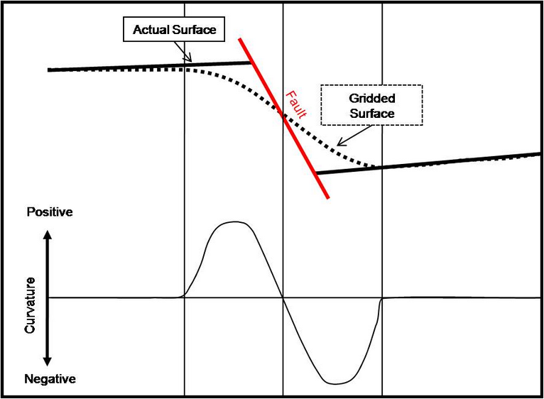
The Compute Grid Curvature Grids tab

Mean Curvature - This operation calculates the average curvature for all azimuth directions. It’s used mostly for deriving other curvature attributes, and isn’t particularly useful for geological interpretation

Gaussian Curvature - This operation calculates the product of the minimum and maximum curvatures. Though it’s been suggested that this method is useful for faults (Lisle, 1994; Wen & Townsend, 1997), Roberts (2001) states that the Gaussian curvature switches between positive and negative values too often to be useful. Though this sign-switching problem could be mitigated by using the absolute values, Gaussian curvature is mostly used for deriving other curvature attributes.

Maximum Curvature - This operation calculates the highest curvature for every point regardless of azimuth or sign. Points with large positive values here have convex curvature, while the negative values reflect concave curvature at some azimuth. Roberts (2001) suggests that maximum curvature is useful for outlining faults and fault geometries.

Without any faults drawn in the overlay, Petra’s gridding algorithms attempt to create a continuous surface between the data points. As such, gridding will inherently smooth over faulting, which creates regions of higher curvature.  Upthrown sides of faults exhibit a positive curvature while downthrown sides have negative curvature. In theory, the zero crossing between the positive and negative curvature is the center of the fault.

Faulting calculated from grid curvature. Modified from Roberts (2001)

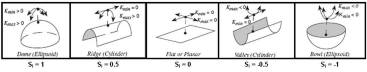
Minimum Curvature - This operation calculates the smallest, flattest curvature for every point regardless of azimuth or sign. Points that still have fairly large minimum curvature values can indicate possible fractures and faults.

Most Positive Curvature - This operation calculates the highest positive (convex) curvature regardless of azimuth. As mentioned earlier, convex structures can be tied to the upthrown sides of faults.

Most Negative Curvature - This operation calculates the highest negative (concave) curvature regardless of azimuth. As mentioned earlier, convex structures can be tied to the downthrown sides of faults.

Dip Curvature - This operation plots curvature in the direction of maximum dip. Effectively, this curvature is a measure of the rate of change of dip in the maximum dip direction. This tends to exaggerate local relief on the structure, which can enhance differential compaction on channel sands and debris flows (Roberts, 2001)

Strike Curvature - This operation plots curvature in the direction of strike. In other words, this measurement highlights ridges and valleys along strike, where positive numbers reflect a ridge and negative numbers reflect a valley. Typically, this operation is used in topographic terrain analysis to help analyze gravity-driven processes like soil-erosion and drainage. More specifically, this method better illustrates where valleys will aid drainage and where ridges will block it. In an oil & gas industry setting, strike curvature can be turned upside-down to help illustrate how the top surface of a reservoir will aid or block the migration of hydrocarbons (Roberts, 2001). In other words, a ridge of positive curvature at the top of a reservoir will act as a conduit for migration, while a valley digging into the top of a reservoir will block migration.

Curvedness - This operation plots the magnitude of curvature independent of shape. This gives a general measurement of the total curvature present within the surface.

Dip Angle (Slope)  - This operation calculates the angle of dip for each point.

Dip Azimuth (Direction) - This operation plots the azimuth of dip. Rapid changes in this may indicate faulting or lineaments.

Shape Index - This operation calculates the Sharpe Index (Si), which is a numerical measurement of shape. The Sharpe Index ranges from -1 to +1, where -1 indicates a point that is shaped like a bowl, 0 is perfectly flat, and +1 is dome shaped. Values between -1 and 0 are valleys, while values between 0 and +1 are ridges. Geologically, this index can be used to emphasize subtle faults or lineaments.

The Sharpe Index. Modified from Roberts (2001)

Output Grid Title - This entry sets the title of the created grid.

Options tab

The Options tab sets a few additional options for the curvature calculation

The Compute Grid Curvature Grids tab

Smoothing

Apply Smoothing Filter Using - This option applies a rolling average to the calculation.  The entry specifies the total number of points to include in the rolling average.  

Resolution of Analysis

Number of Rows (Cols) Btwn Samples - This option decimates the data to only analyze every N’th sample.  Setting this value to 2, for instance, would only calculate the curvature on every other grid node.  Setting this value to 5 would only load every 5th sample.  By default, this option is set at 1 to analyze every grid node on the selected grid.

Normalization

Normalize Output Grid From - This option converts the values calculated by the curvature calculation to instead use a user-specified minimum and maximum.  This can be useful for better illustrating some grids that normally would have a gradient too small to usefully display on a grid.

Convert Negative Surface to Positive Values - This option simply applies the absolute value of all surface calculations.  With this option, Petra will substitute a positive value for negative values.

Output Azimuth as... - This option changes how Petra exports azimuth values.  This can be useful for exporting grids to other software packages that handle azimuth a little differently.

Reference tab

The Reference tab simply provides the reference for the curvature calculations.

The Compute Grid Curvature Grids tab