|
The Raster Calibration utility provides options for straightening, depth calibrating, and digitizing a raster image; you can also pick formation tops and pay intervals. It is a quick way to view a raster log without using the Cross Section Module.
To import un-calibrated raster logs:
- On the Main Module, select the Rasters tab.
- Click the Calibrate
button to open the Calibrate Log Image tool.
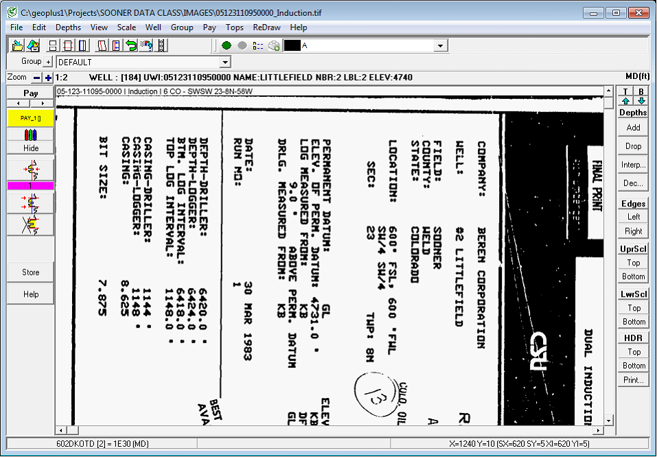
- Select the button on the toolbar. Alternatively, select File > Open on the menu bar at the top of the screen. Next, navigate to folder containing the images and select the desired image file. By default, Petra will look in the the projects IMAGES folder.
Its usually worthwhile to spend a few seconds scrolling up and down through the image to see whats actually there. Usually, raster images store a complete copy of the scanned paper log, which can contain the same log at different scales as well as repeat sections.
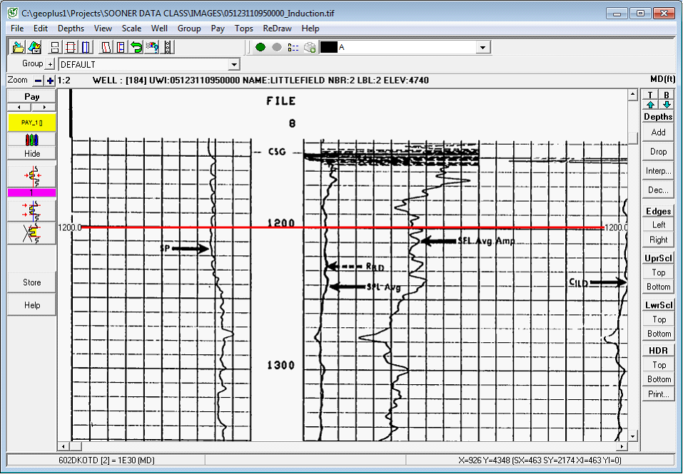
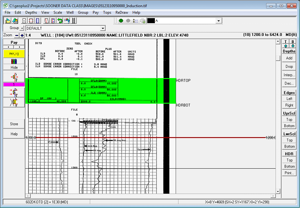
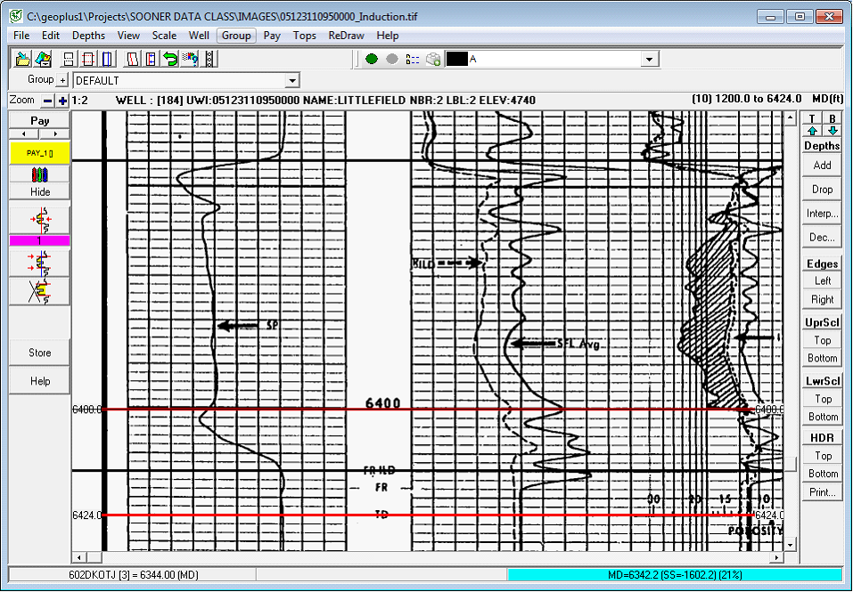
- A scanned log is just an image, so Petra needs a way to know how the image corresponds to depth. Select the Add button on the right side of the screen; note that this turns the mouse pointer into a line. Click right on the 1200 marker, and enter in the depth.
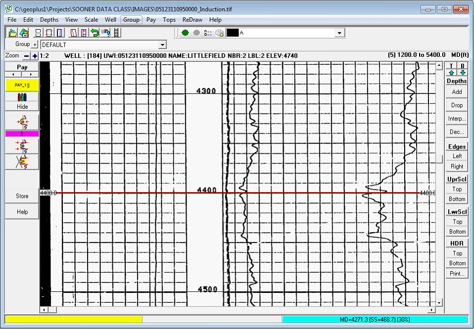
- Scroll down the image to 5400MD, and add another depth calibration point. Notice that Petra automatically extrapolates depths between two depth points, which are marked with thin black lines. Commercially depth-calibrated logs often have dozens of calibration points, most of which are unnecessary. Well-scanned logs that minimize image stretch really only need a few points. In our case, the calibration is pretty good for most of the depth range, but could use improvement. Add more depth calibration points where the calibration is off (around 2400MD and 4900MD).
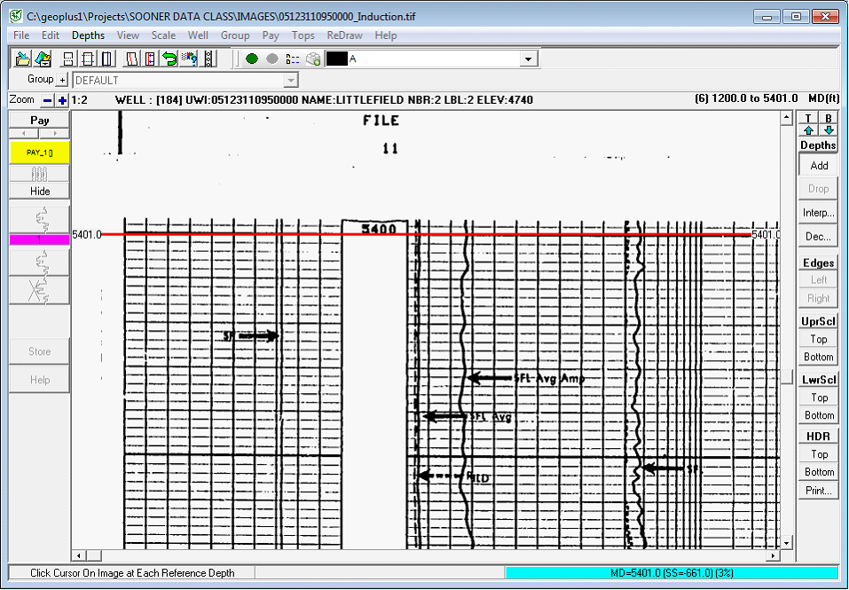
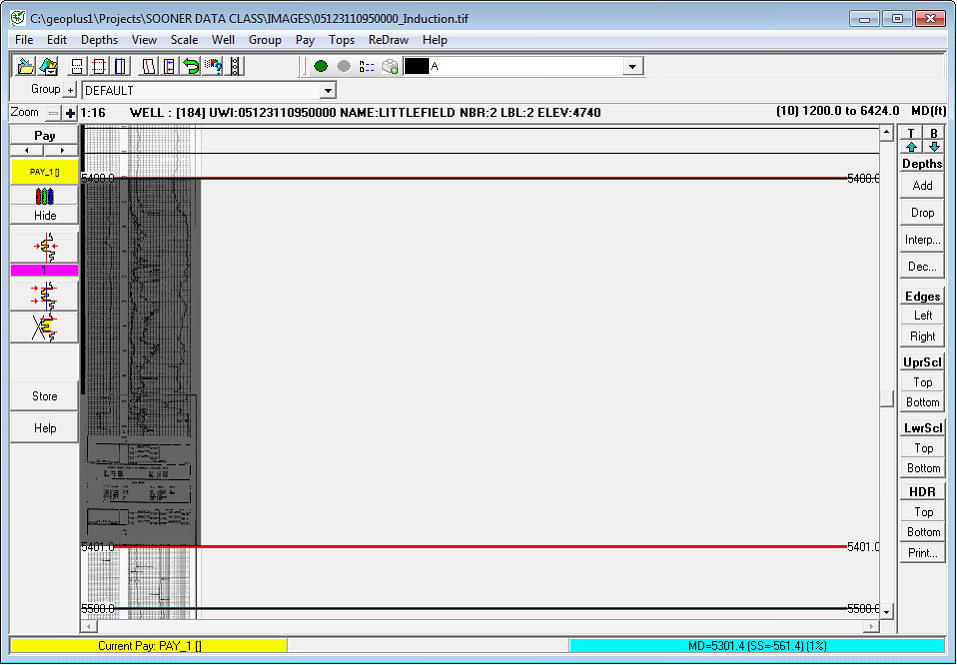
- Now that the top part of the well is calibrated, scroll to the 5 section, and add a calibration point just a little below the 5400MD line. Put the depth in as 5401MD.
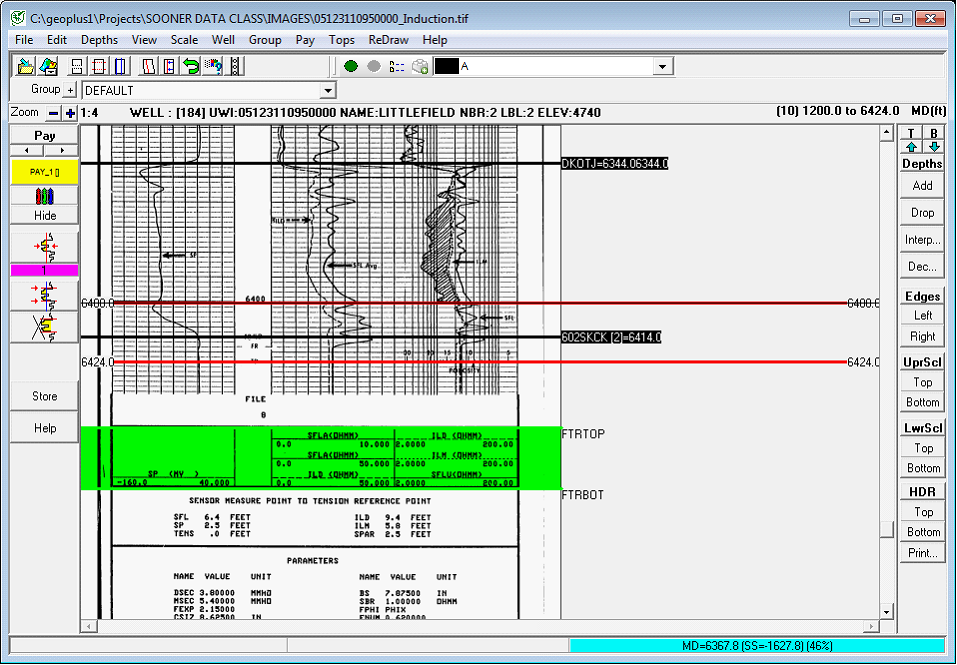
- Add a point at the TD marker at 6424MD and at a few more points to get a good calibration to the image. Again, add depth calibration points where the black lines are off the 100 intervals on the log. Notice that Petra will add thick black lines in the correlation these are actually the tops we imported earlier.
- Select the - button to zoom out on the section. Right now, we have two sets of depth calibration points over the image: a shallow set over the 1 log, and a deeper set over the 5 log. In between, theres a lot of extraneous information that wed rather just cut out. Select CTRL and click somewhere in the region between the shallow and deep set of calibration points. Notice that the section goes dark, signifying that it wont display on cross sections. In our case, this will just keep the entire section from being crammed into a tiny sliver between 5400MD and 5401MD, but this technique can be really useful to cut out other extraneous parts of an image. This technique is also useful for cutting out a repeat section between one run and the next.
- Select the + button to zoom back into the image. The next step is to add scales. Petra can draw both an upper scale and a lower scale on the same cross-section. Scroll to the bottom of the depth calibration points. On the LwrScl section, select the Top and Bottom buttons to set the boundaries of the upper scale marker.
Next, scroll to the top of the image. On the UprScl section, select the Top and Bottom buttons to set the boundaries of the upper scale marker.
- Scroll to the very top of the image. Add the top and bottom of the header with the Top and Bottom buttons in the HDR section.
- The final step is to add a group name. Group names usually describe the depth-calibrated part of the image usually by describing the scaling or the curves. Right now theres only one group name DEFAULT. On the menu bar at the top of the screen, select Group>Add or Delete Groups.
From a user-perspective, group names are a way of comparing similar raster images from one well to another. Though commercial vendors generate thousands of unique group names for every combination of tool and scale, its usually better to have fewer, more general group names rather than many excruciatingly exact ones. In the Image Group Name entry, type in Induction, and select the Add button.
- Select the Done button. Back in the Calibration tool, use the group name dropdown and select Induction. Select the
 button to save the calibration to the group name. Behind the scenes, Petras actually creating a LIC file that saves these calibration points the location of which is shown in the Save File As window. button to save the calibration to the group name. Behind the scenes, Petras actually creating a LIC file that saves these calibration points the location of which is shown in the Save File As window.
|