The Log Correlation Tool is an easy way to correlate formation and unassigned tops as well as faults and pick pay intervals.  To open the Log Correlation Tool, click the Log Correlation icon on the toolbar in the Main Module:  

Introduction to Log Names and “Log Types”

The fundamental problem with log data is the proliferation of log names created by different commercial data vendors and individual users.  The same general type of curve (such as a gamma ray curve) can have hundreds, if not thousands, of different names in a single project.

The Log Correlation Tool gets around this problem by using “Log Types.”  A Log Type is just an alias list of equivalent logs.  In the example below, the “Resistivity” Log Type we build will contain a list of the resistivity raster logs in a project.  To display a resistivity curve on a cross-section, we simply tell Petra to draw the “Resistivity” Log Type.  Petra then goes down this list of raster logs for each well on the cross-section and draws the first one it finds.  For the interpreter, this means that time invested in setting up Log Types will pay off with quicker, easier cross-sections later.

Guide

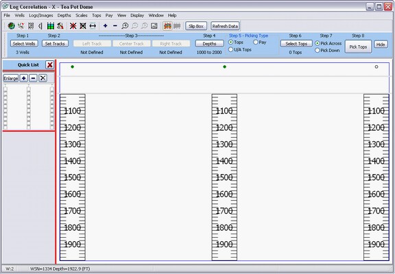
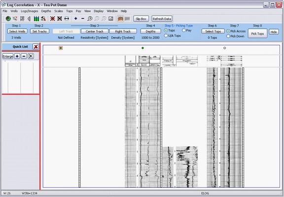
The guide at the top of the screen shows the suggested workflow for using the Log Correlation Tool.  You’ll want to select a few wells, set the Log Types for each column, put raster and digital logs inside those Log Types, set the depths, and finally select and pick tops and pay intervals.  The Quick Guide on the top of the screen has a set of buttons that link directly to these different tasks in this order.

Step 1 - Select Wells

There are two ways to select wells: with the Map Module or directly from the Cross Section Module

With the Map Module - The “Select Wells” button on the guide takes you directly to the Map Module.  Alternatively, click the map icon at the top of the screen: .  Once in the Map Module, select individual wells with the left mouse button to add wells to the Log Correlation Tool.  Right click to stop and switch back to the Log Correlation Tool.

With the Cross Section - Select Wells>Use Cross Section Wells.  This option selects the wells used in the Cross Section Module.

In the example below, there are three wells with no log types selected.  The default depths for the module are from 1,000’ to 2,000’ MD.

Step 2 – Set Columns

The next step is to set the columns with either the “Set Columns” button on the guide, or the “Set Columns” button on the toolbar:  .  Columns simply define where raster and digital logs will be drawn in relation to the well symbol and data posting.

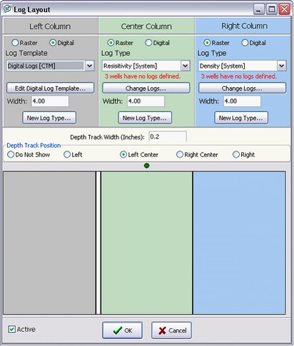
To define a column, first define whether the column will contain digital or raster log data.  Next, click the drop down box directly under “Log Type” for each column.  Under this drop down menu, notice that Petra initially creates a few default Log Types including Density, Gamma Ray, Induction, Neutron, Resistivity, and Sonic.  In this example, the Resistivity Log Type will be drawn in the center column, and the Density Log Type will be drawn in the right column.  You can also select the “New Log Type” button on the lower right corner of this screen to create a new Log Type.

You can also modify the location of the depth track.  The depth track plots MD or TVD depths next to the raster logs.  This option simply moves the location of the depth track relative to the other columns and the well symbol.  In the example below, notice that the depth track is set to “Left Center” between the center and left column.

Notice the text underneath each of the raster columns initially reads “3 wells have no logs defined.”  Initially, none of the Log Types have any logs names assigned to them.  In other words, Petra doesn’t know what raster log names (also known as “group names”) should be drawn in either the “Resistivity” or “Density” columns.  The next step is to assign specific logs to the Log Types.  

Click OK to go to the Log Correlation Tool main screen.  Alternatively, click the “Change Logs” button under one of the Log Types to take you directly to the next step at the Assign Log Type screen.

Step 3 - Putting Logs Inside Columns

The Log Correlation Tool can display both digital and raster logs.

Raster Logs

The next step is to put raster logs inside the newly defined columns.  Practically, this means that we need to assign raster group names to the Log Types.  In the main screen, select one of the defined columns under Step 3.  In this example, the center column with the Resistivity Log Type is selected.

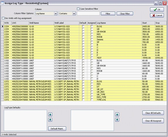
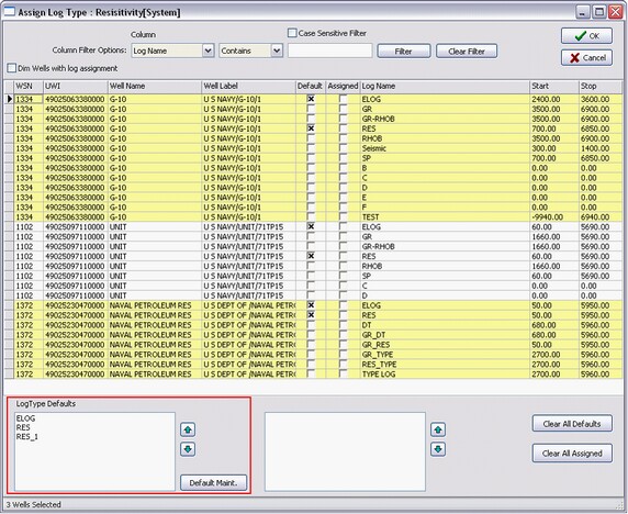
This brings up the Assign Log Type screen.  This screen shows the available raster logs and their start and stop depths for each selected well, with shading separating different wells.  You can sort by ascending or descending order for each column.

This screen also features a search box at the top of the screen that filters data by WSN, UWI, well name, well label, log name, or start and stop depths.  Select “Filter” to return the data meeting the criteria.  This filter can also be made sensitive to capitalization by selecting the “Case Sensitive Filter” box.  After narrowing your logs and wells by applying one filter, you can select different criteria and select “Filter” again to further limit the results.  “Clear Filter” removes all filtering and returns all the available raster logs for all selected wells.

You can select raster logs for the wells either by aliasing default raster groups to a Log Type or by individually assigning raster logs for each well.  Using both approaches together will give the best combination of speed and customization.  A good Log Type “default” list is a useful “top-down” way of making a quick first pass at the proper raster log for each well, while assigning individual logs ensures (in a “bottom-up” way) that you are displaying the best possible log.

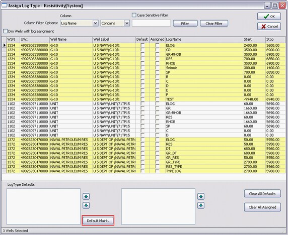
“Default” Log Type Rasters  – This method aliases different raster groups to one Log Type.  Petra then assigns a “default” raster log to the well based on this list.  In this example, different resistivity raster images will be aliased to a single default “Resistivity” Log Type.  The first step to setting up a Log Type is to select the Default Maintenance button on the lower left side of the screen (highlighted in red).

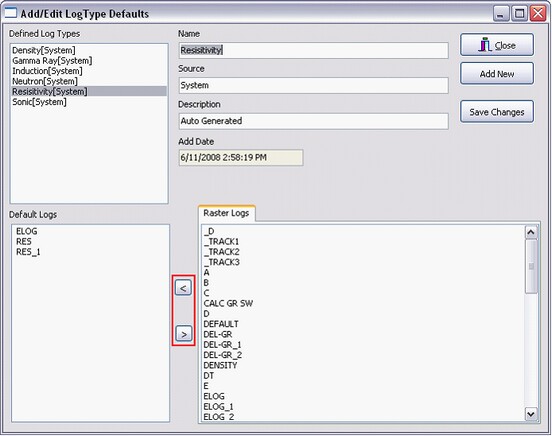
This brings up the Add/Edit Log Type Defaults screen.  Here you can add, delete, or modify the existing Log Types.  In this example, the Resistivity type is selected in the “Defined Log Types” box in the upper left corner.  Next, select the raster names to add to the Log Type.  To add or remove raster names to the Log Type, select the “<” or “>” buttons (highlighted in red).  In the example below, the Resistivity Log Type will bring up the Elog, Res, and Res1 raster logs as a default.  In essence, Petra will try to draw the first available raster log on this list for the Resistivity Log Type in the center column. Click Save Changes and Close to exit.

Back at the Assign Log Type screen, notice that the raster logs selected on the default Log Type list now show checks in the boxes underneath the “Default” column.  In addition to showing which logs are selected, these check boxes can also be used to quickly add and drop logs from the selected Log Type.  For example, clicking the “Default” check box next to the “ELOG” raster log will drop it off the “Resistivity” Log Type for all wells.  Clicking the same “Default” check box again restores it to the list.  The Log Type Defaults list (highlighted in red below) shows the order of the default logs for the selected wells.  Again, log names higher on the list will be drawn before log names lower on the list.  To change the priority of the alias list, select a log name and use the and buttons.

“Assigned” Individual Raster Logs - The other way of selecting raster log names to display is to individually assign raster logs for each well.  Though this process takes more time, assigning individual logs allows you to select the best raster log for each well.  Petra stores this information for the next time you bring the well into the Log Correlation tool.

The easiest way to assign a specific raster log to a well is to use the Assign Log Type screen.  To select a specific raster log, select that raster log’s check box in the “Assigned” column.

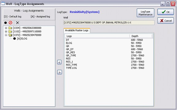
Additionally, you can also open the well-specific “Log Type Assignments” box by double-clicking an individual well.  To assign a raster log to the selected well, select the specific raster log from the “Available Raster Logs” list on the right side of the screen and click the “<” button.  In the example below, the “ELOG” raster has been assigned to the selected well.  Select OK to save the changes and return to the main “Assign Log Type” screen.

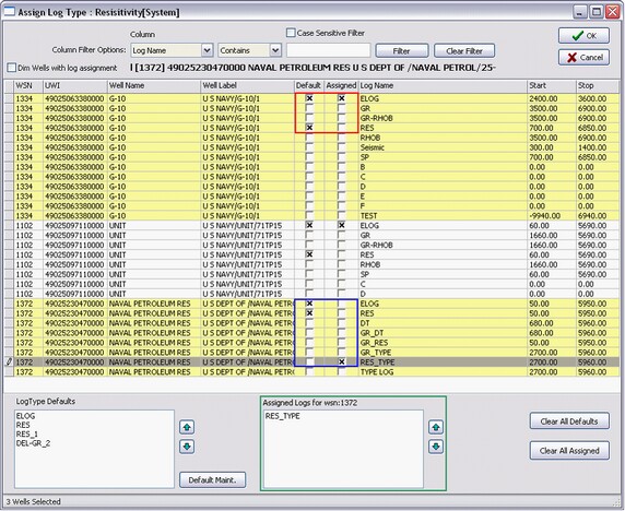
In the example below, notice that the two different wells have “assigned” logs.  In one case (highlighted in blue), the log RES_TYPE will be plotted instead of the two default logs, RES and ELOG.  In the other case (highlighted in red), ELOG is both a default log and an assigned log.  This just means that it will be displayed regardless of its order in the default Type Log list.

The Assigned logs box (highlighted in green below) shows the assigned logs for the selected well.  If a well has multiple assigned logs, you can prioritize them with the and buttons.  Log names at the top of the assigned logs list will be shown before log names at the bottom of the list.

After setting up one Log Type, this is a good place to go back and repeat the same Step 3 in order to fill the log types established for the columns in step 2.  Carrying on with the example, the screenshot shows the results of setting up log types for resistivity and density logs.  Notice that the far left well does not have a log.  This is because the depth scale is still from 1000-2000’ MD, which is above the start of that well’s raster logs.

Digital Logs

In addition to raster logs, Petra can display digital logs inside the Log Correlation Module.  While raster logs are simply images with fixed scales and curves, digital logs actually contain the actual numerical values recorded by the tool in the wellbore.  Digital logs are much more flexible and can be displayed at any curve scale and in any combination.

To change the display of digital logs, select one of the digitally-defined columns on the guide under Step 3.  In this example, the left column with the “Digital Logs” log type is selected.  This brings up the LAS to Raster screen.

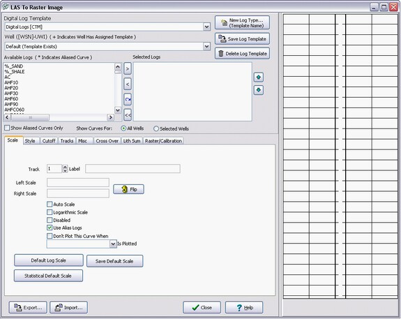
Petra uses a digital log “template” containing scales, colors, and position information to draw the digital log curves on the main Log Correlation Tool window.  A template is established for each Log Type.  In this example, the “Digital Logs” Log Type is selected, and is shown on the digital Log Template dropdown menu (highlighted in red).

You can select digital logs for the wells either by creating a default template for a Log Type or by individually assigning log templates for each well with the “Well” dropdown menu (highlighted in blue), which  switches between the Default digital log template and the templates for the wells selected in the Log Correlation tool.  This works similarly to the “Default” and “Assigned” raster logs discussed earlier.  Though you can create digital log templates for each well, it’s probably much faster to use a single default log template with aliased digital logs.

“Default” Digital Log Template – This method uses a single template of digital logs and display options for all wells.  This method works particularly well with digital log aliasing, which establishes a list of curve names that are equivalent.  In the example project, gamma ray curves are stored as GR, GRN, GRR, and GRS.  Once those curve names are aliased to the single curve name “GR”, the digital log template treats them all as equivalent.  For most projects, there’s no need to use individually assigned digital log templates to deal with different curve naming conventions.  Once the curves and display options are set, make sure the “Default” option is selected on the Well dropdown menu (highlighted in blue) and select “Save Log Template.

“Assigned” Individual Templates – With a robust digital log aliasing scheme, the only real reason to use individual digital log templates is to use different scales or other display features (such as color or shading) for different wells.  Once the curves and display options are set for the individual well, make sure the well’s API/UWI is selected on the Well dropdown menu (highlighted in blue) and select “Save Log Template.”

The “Available Logs” list on the left side of the screen gives a list of all digital logs that can be added to a well.  Note that aliased curves are annotated with an *.  This list can be filtered to include the digital logs from all wells in the project, or just the wells currently selected in the Log Correlation Module.  To add a log, highlight the name in the "Available Logs" list and click the add button (">").  This moves the log over to the “Selected Logs” list.   To remove a log, highlight the log name in the “Selected Logs” list and click the remove button ("<").

Once a log is added to the “Selected Logs” list and is highlighted, the track and display options for that log can be set on the various tab screens. Each displayed log has its own scale and color settings established by the Scale through Raster/Calibration tabs on the bottom of the Las to Raster Image box. For a more detailed walkthrough of displaying digital logs, see “How to Display Digital Log Data.”

Scale tab - The Scale tab governs a few basic settings for each log.  The Scale tab also sets the left and right scale for the selected log, as well as if the log will use the alias list.

Style tab – The Style tab changes how the selected log is displayed.  This tab sets the color and thickness of the curve, as well as any shading.  Shading can highlight log values above or below a cutoff value, or change color as a function of another log (GeoColumn shading).

GeoColumn Shading – When the GeoColumn option is set on the Style tab, the GeoColumn tab appears.  GeoColumn shading colors the area between a curve and the track edge with variable color based on log curve values.  The color shading under the curve can either based on same curve or from an entirely different curve.  This shading can either fill to the left or right edge of the track.

Tracks tab – The Tracks tab controls how the background grids are drawn for the digital logs.  This tab sets the width of the tracks and configuration of vertical scale lines.  Double clicking each track name under the Track Definitions box toggles the depth track on and off.  Hidden tracks (denoted by the   symbol) don’t show grids or any curves.  

Misc tab – The Misc tab sets a few additional options regarding digital log display.  Plotting track grids after log curves layers the track grids over the log curves for additional visibility.  Using curves from other well completions will use curves from wells with a similar API/UWI number (ending in 00001, 00002, etc).  Plotting the shading between logs after other shading will plot this shading on top of any other curves for visibility.  Display Curve units in header will show the curve units stored in Petra’s database (on the Logs tab in the Main Module) on the curve header.  Show aliased curve name in track header label will show the curve’s actual name instead of the aliased name.

Crossover – The Crossover tab shades the space between two log curves or between a curve and a track edge.  Crossover shading is commonly used for illustrating the “gas effect” on porosity logs.  Simply select curve 1 and 2, and whn the shading should appear.  It’s worth noting that cossover shading simply fills in the area between the two curves as drawn on the track, and does not require the two curves to be at the same scale.

LithSum – Lith summaries are useful for displaying cumulative data.  As an example, if a sample has 70% shale and 30% sandstone, it’s generally more useful to represent these two numbers as a cumulative plot adding up to 100 instead of two separate curves at 30 and 70.

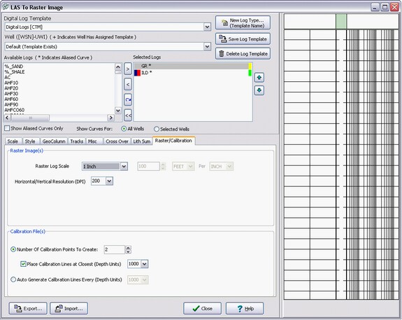
Raster/Calibration – The Log Correlation Module actually creates a temporary raster image of the digital log for display.  This tab governs how this temporary file is created.  The Raster Image section sets the overall resolution of these raster images.  If images are blurry, try adjusting the log scale to be more in line with the scale on the mail Log Correlation Module.  Adjusting the DPI can also sharpen the image, but at the cost of slower drawing.

Normally, the Log Correlation module draws logs with a linear scale between the top and bottom of the digital data.  Deviated logs, however, don’t have a perfectly linear relationship between MD and TVD.  Adding additional calibration points helps to stretch and squeeze the temporary raster image to better represent a TVD log.  Note that adding additional calibration points requires more drawing time.

Step 4 - Depths

The next step is to set the depths for the correlation tool.  In the main screen, click the “Depths” button on the guide, or click the depths button on the top toolbar: .

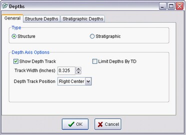
Depth Type

The depth type can be either "Structure" or "Stratigraphic". A structural cross-section has a depth interval defined by measured or SubSea depths.   A stratigraphic section instead has depths defined with formation tops, where the raster logs are hung on the upper fm top.  Stratigraphic cross-sections are useful for showing variation in stratigraphy independent of structural change.

Depth Axis Options

Show Depth Track – This option toggles the display of the small track that shows MD, TVD, or SS depths.  To hide it, deselect the “Show Depth Track” option.  Hiding the depth track will also hide any perf and test information.

Limit Depths By TD – This option limits the drawn raster logs and the depth track down to a well’s TD (as stored in Petra’s database) rather than to full extents of the bottom set with the Structure or Stratigraphic Depths tabs.

Track Width - This governs the width of the depth track.  Text inside the depth track is automatically scaled.  Expanding the width of the Depth Track can make the measured depth numbers easier to read.

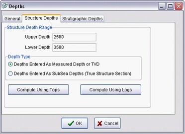
Structure Depths

If the plot is structural, use this tab to set the depths.  Enter the "Upper Depth" and "Lower Depth" values to define the desired section to display.  Depth values can be entered as either measured or SubSea depths.  Remember that SubSea values below sea level (like those on wells drilled on the Gulf Coast) are negative numbers.

Compute Using Tops – Petra can automatically compute a valid structure depth range from the tops selected for the cross-section.  If no tops are picked for the selected wells, Petra won’t be able to calculate a depth range.

Compute Using Logs -  Petra can automatically compute a valid structure depth range from the logs selected for display.  Here, PERA will calculate depths that will cover the top of the shallowest and bottom of the deepest logs.

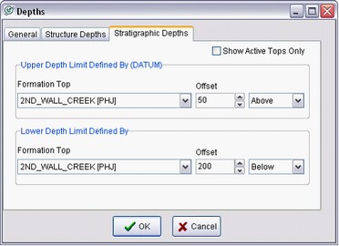
Stratigraphic Depths

If you’ve selected stratigraphic depths, use this tab to set the scaling.  Select the formation tops which define the upper and lower depth. Petra will flatten the wells along the upper formation.  You can also add an "offset" number, which allow stratigraphic depths to include data a set number of feet or meters above and below the selected tops.  It’s also acceptable to use the same formation top for both the upper and lower depth limits with a sufficient offset above and below, as in the example below.  Notice that the upper and lower depth limits are set by the same top with offsets 50’ above and 200’ below.

It’s worth noting that if either of these formation tops are null for a well, Petra doesn’t have anything to flatten on and the well will be blank.  For initial correlation work, it is generally best to pick a consistent, widely correlated top to flatten on.

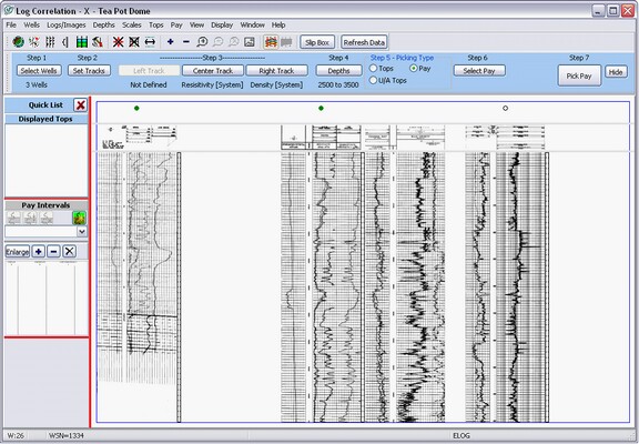
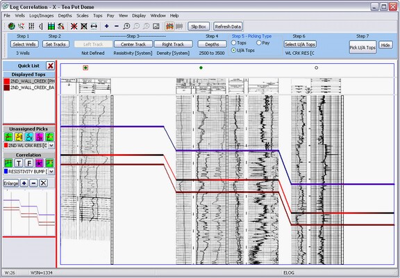
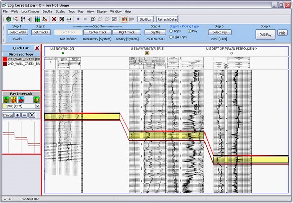
At this point, the cross section shows the raster logs at the specified depths.  In the example shown below, the cross-section shows the resistivity logs in the first column and density logs in the second column.  The depth scale is from 2500’ MD to 3500’ MD.

Step 5 – Select Picking Type

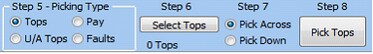
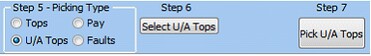
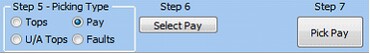
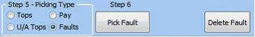
The previous steps simply create a cross-section to interpret.  The next step is to select the pick type.  These three buttons on the quick list are an easy way to switch between picking tops, unassigned tops (“U/A Tops”), pay intervals, or  faults.  Each “picking type” button under Step 5 changes Steps 6, 7, and 8 to reflect the particular pick type.

Each pick type changes the Quick List on the right of the screen, as well.  The Quick List is the most convenient way to pick tops, pay, and faults.  To toggle the Quick List on and off, click the button in the upper left corner of the screen, or select View>Quick List on the menu bar at the top of the screen.

Picking Fm Tops

The Log Correlation Tool allows you to create and store formation tops.  Formation tops reflect distinct, mapable lithostratigraphic units that are equivalent from well to well.  Formation tops are stored to Petra’s database, and are shared among different modules and different users.

Step 6 - Formation Tops Display Options

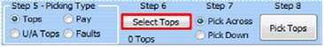
The next step is to select the tops you want to display and pick.  First, select the “Tops” option under the Step 5, and then click the “Select Tops” button under Step 6 on the guide (highlighted in red).

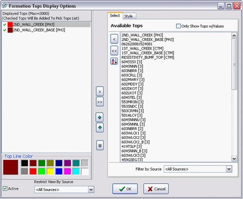
This brings up the Formation Tops Display Options window.  To display a formation top in the Log Correlation Tool, first select it on the “Available Tops” list and click the “<” button to bring it over into the “Displayed Tops” list.  The tops listed in the Available Tops list can be filtered to show only the tops with values for the wells in the Log Correlation tool or by source.

Once on the Displayed Tops list, you can change the color of the top as it shows up on the plot. The small check box next to the name on the Displayed Tops list toggles whether the picks are for display only or can be modified.  Tops with a green check can be picked and shown up on the Pick Tops list, while those without a green check are display only.

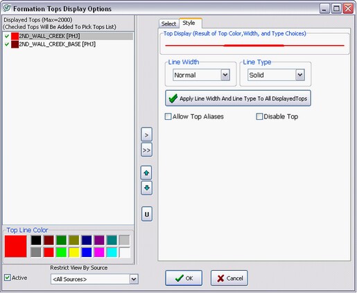
After the tops are selected, the next step is to pick the style of the displayed tops.  Under the Style tab, you can change how the line between tops is drawn.  Line width makes the lines between tops thicker and thinner, while the line type determines whether the line is dashed or solid.  The “Apply Line Width and Line Type” button will change the width and type for every other displayed top, but will retain each line’s color.  In the example below, the “2nd Wall Creek” top is selected.  The style tab shows that this top is red, solid, and of normal width.

If your project has Top Aliases set up in the Main Module, click the “Allow Top Aliases” to use them.

“Disable Top” temporarily hides the specific formation top on the cross-section while retaining its display settings.  Disabled tops will have a symbol next to their name.

Step 7 – Pick Fm Top Style

When the “Tops” picking type is selected, Step 7 shows the two options for picking formation tops: across and down.  You can change the pick style with the buttons on the Guide, or by using the and buttons on the Pick Tops part of the Quick List.

Pick Across – This is the standard pick mode in the Cross Section module.  In this mode, a single formation top is picked across all wells shown.

Pick Down - In this mode, tops are picked in the order they’re shown on the Pick Tops list.  Practically, this means that tops can be picked successively down the same wellbore before moving to the next wellbore.  It helps to have the tops in a stratigraphically successive order going down the wellbore on the Pick Tops list.  Use the buttons to move a selected top up or down in the Pick Tops list.

Step 8 - Picking Fm Tops

Selecting “Tops” on step 5 changes the Quick List to Pick Tops mode.

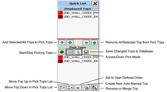
To start picking tops, first select the desired fm top on either the Displayed Tops list at the top or the Pick Tops list at the bottom.  Next, select the “Pick Tops” button on the guide or the green button on the Pick Tops Quick List: .

Remember that the two pick modes work differently.  “Pick Across” creates a single top across all wells, while “Pick Down” cycles through the Pick Tops list.  To create fm tops, just click the depths on the raster logs where your tops are located.  To stop picking, right click the mouse or click the stop button on the Pick Tops Quick List: .  The example below shows formation tops for the top and base of the 2nd Wall Creek in red.  Notice that the currently active fm top, 2nd Wall Creek, is shaded to black.

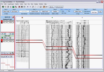
You can also create “Auto-named” fm tops using the Create New Fm Top button: on the Quick List.  Just like regular tops, auto-named tops correlate across logs and can be used in cross-sections and the map module.  The only real difference is that the normal fm top setup is bypassed, so auto-named tops are named on the current date and time - DDMMYYYYHHMMSS.  In the example below, the auto-named top “10082008143211” just means it was created 8 October, 2008, at 14:32:11 (2:32:11PM).  Auto-named tops are great for quickly correlating an unknown surface, and setting the name and source later.  Additionally, auto-named tops can easily be merged into existing fm tops.

Renaming and Merging Tops

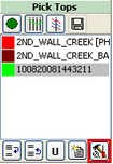
Merging tops takes essentially takes the values of one named set of tops and moves them to another named set.  Instead of dealing with two tops representing the same surface, it’s more convenient to merge them into one.  To merge the two together, first select the top to merge into another and select the “Rename/Merge Selected Top.”   In the example below, the “10082008143211” auto-named top is selected.

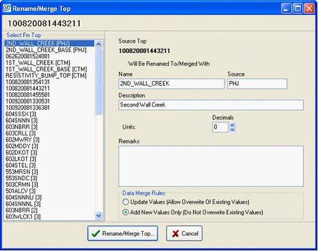
This brings up the Rename/Merge Top screen.  Notice that the Source Top is listed at the top of the screen.  This is the top that will be renamed or merged into the top selected on the list at the right of the screen.  In this example, the “10082008143211” auto-named top will be merged with the 2nd Wall Creek.

The Data Merge Rules settings at the bottom of the window set how the two tops will be merged together

Update Values – In wells where both tops exist, the source top (in the example below, 10082008143211) will remain and the selected top (2nd Wall Creek) will be erased.

Add New Values Only – In wells where both tops exist, the selected top (in the example below, 2nd Wall Creek) will remain and the source top (10082008143211) will be erased.

Picking Unassigned Tops

The Log Correlation Tool also allows you to create and store “unassigned tops.”  There can be multiple unassigned tops with the same name on the same well.  Because of this, unassigned tops are useful for correlating things outside the traditional definition of a formation top.  This can include possible faults or other marker "picks" that are considered by the interpreter to be unknown, uncorrelated or otherwise "unassigned".  Unassigned tops can be easily correlated and converted into formal formation tops.  Unassigned tops are stored to Petra’s database, and are shared among different modules and different users.

Step 6 - Formation Tops Display Options

Just like regular formation tops, you also need to turn on the display of unassigned tops.  First, select the “U/A Tops” option under the Step 5, and then click the “Select Tops” button on the guide (highlighted in red).

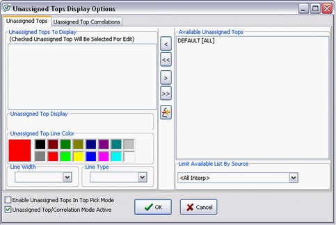
This brings up the Unassigned Tops Display Options Screen.  This screen shows all the pre-existing unassigned top names in the project.  In the example below, there is only the “default” unassigned tops name.

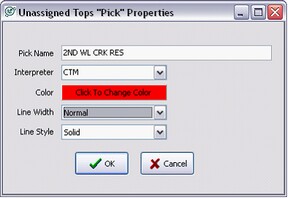
Since this will be shared throughout the whole project, it’s a good idea to make a new, named set of unassigned tops.  To create a new set of unassigned tops, select the button.  On the Unassigned Tops “Pick” Properties box, enter a name under “Pick Name” that reflects the purpose of your unassigned tops.  This can be as generic or as specific as you like.  In the example below, the picks are all going to be on 2nd Wall Creek resistivity features, so the pick name is “2nd Wl Crk Res.”   Next, select or enter an interpreter name.  It’s a good idea for every interpreter to have their own in order to prevent one user from overwriting another user’s work.  In the example below, the source name is “CTM.”    Next, select the line style, width and color for the unassigned tops.  Select OK to create the correlation and return to the display options screen.

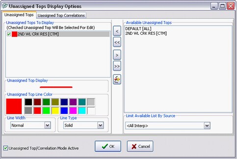
Notice that the unassigned tops name now appears in the Available Unassigned Tops list on the right of the screen.  To display a formation top in the Log Correlation Tool, first select it on the Available Tops list and select the “<” button to bring it over into the “Unassigned Tops To Display” list.

Once on this list, you can still change the color of the unassigned tops. Selecting the small check box next to the name on the Unassigned Tops To Display list toggles whether the picks are display only or can be modified.  Tops with a green check can be picked and modified in the correlation tool, while those without a green check are display only.

Step 6 Cont.  - Unassigned Top Correlations Display Options

Unassigned tops by themselves have no relationship to each other.  Correlating unassigned tops links them together across wells into a single named unit.  These correlations can be flattened to show stratigraphic variation or converted into regular formation tops.  One of the best uses for correlation is to flatten the cross section on localized distinctive log features with no formal name.

Just like regular formation tops and unassigned tops, you also need to turn on the display of unassigned top correlations.  First, select the “U/A Tops” option under the Step 5, and then click the “Select Tops” button on the guide (highlighted in red).

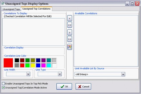
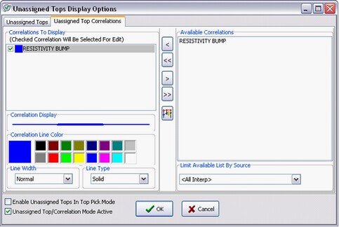
This brings up the Unassigned Tops Display Options Screen.  To look at correlations, click on the “Unassigned Top Correlations” tab on the top of the screen.  This screen shows all the pre-existing unassigned top and unassigned top correlations in the project.  In the example below, there are no available correlations. To create a new set of unassigned tops, select the button.  

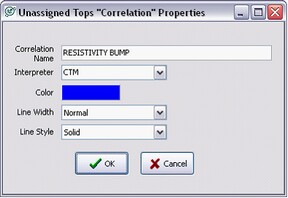
On the Unassigned Tops “Correlations” Properties box, enter a name under “Correlation Name” that reflects the purpose of your unassigned picks.  This can be generic or specific as you like – in the example below, the correlation is on a single resistivity bump above the 2nd Wall Creek, so the correlation’s name is “Resistivity Bump.”  Next, select or enter an interpreter name.  It’s a good idea for every interpreter to have their own to prevent one user from overwriting another user’s correlations.  In the example below, the source name is “CTM.”    Next, select the line style, width and color for the unassigned top correlation.  Select OK to create the correlation and return to the display options screen.

Notice that the correlation now appears in the Available Correlations list on the right side of the screen.  To display a correlation in the Log Correlation Tool, first select it on the Available Tops list and click the “<” button to bring it over into the “Unassigned Tops To Display” list.

Clicking the small check box next to the name on the Correlations To Display list toggles whether the correlations are display only or can be modified.  Tops with a green check can be picked and modified in the correlation tool, while those without a green check are display only.

Step 7 - Picking Unassigned Tops and Correlations

Selecting U/A tops on step 5 changes the Quick List to show the Unassigned Picks toolbar.

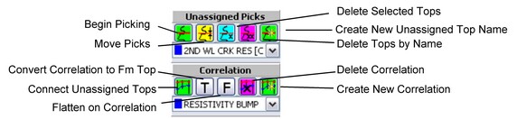
Unassigned Picks

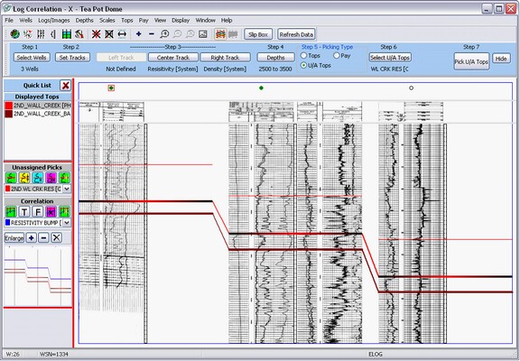
Making Unassigned Tops:    This creates new unassigned tops under the picks name shown in the dropdown menu.  Different pick names can be used to keeps groups of unassigned picks separate by both purpose and interpreter. In the example above, new unassigned tops will be part of the “2nd WL CRK RES” name created earlier.  To pick tops, click on the logs on the main screen.  Multiple unassigned tops with the same picks name can be added to the same wellbore.  Right click to finish picking tops.

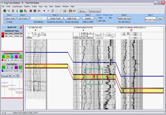
This brings up the option of saving the new pay intervals to Petra’s database. Selecting “No” will erase all new, unsaved unassigned picks.   In the example below, notice the red lines signifying the resistivity anomaly picked as a unassigned top.

Moving Unassigned Tops:  To move unassigned tops, select this button.  Left click the unassigned top to move and drag it to the new location.  When finished, right click the mouse button.  This brings up the option of saving the new unassigned tops to Petra’s database. Selecting “No” will leave all unassigned tops unchanged.

Delete Selected Tops: To delete unassigned tops, select this button.  Left click the unassigned top to delete it.  The unassigned top interval will be hatched with red to show that the changes haven’t been saved to the database.  When finished, right click the mouse button.  This brings up the option of deleting the unassigned top from Petra’s database. Selecting “No” will leave all unassigned top picks unchanged.

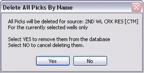
Delete Tops by Name: This button deletes all the unassigned tops with the currently selected unassigned tops name.  In this example, the “2nd Wl Crk Res” unassigned tops group is selected, so selecting this option will delete all the “2nd Wl Crk Res” unassigned tops on the currently selected wells.

Create New Unassigned Tops Name:    This button provides another quick way to create new unassigned group names.  This brings up the New Pay Interval Definition screen.  Enter the name, source, description, and color of your pay zone.  Unassigned top names created here will automatically show up in the Unassigned Picks dropdown menu on the Quick List.

Unassigned Correlations

Connect Unassigned Tops:  This button designates selected unassigned tops to a specific correlation.  First, select the correct correlation name on the lower dropdown menu (in the example above, the correlation is called “Resistivity Bump”).  Next, select the “Connect Unassigned Tops” button and click on unassigned tops on the wells to add them to the correlation.  Right click when done.  The unassigned tops will now be connected by a line to signify that they are part of a correlation.  In the example below, the blue correlation line connects the unassigned tops.

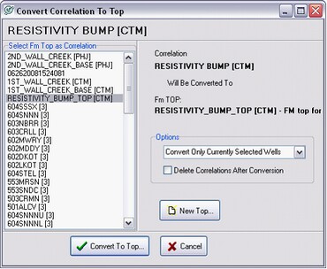
Convert Correlation to Fm Top:  This button converts a correlation into a fm top.  As a formal fm top, the surface can be gridded or used in calculations.  First select the appropriate correlation from the correlation dropdown menu.  Next, select the “Convert correlation to Fm Top” button to bring up the “Convert Correlation To Top” window.

This brings up the Convert Correlation To Top window.  Here, select an existing fm top or create a new top for the correlation.  In this example, the “Resistivity Bump” correlation will be converted to the “Resistivity Bump Top” Fm top.  This newly created fm top will be stored into Petra’s database.

This screen also gives you the option to convert the correlation for all wells in the database, only the currently selected wells in the Log Correlation Tool, or only the wells selected in the Main Module.

Flatten on Correlation:  This option flattens all wells onto the correlation selected on the correlations dropdown menu.  This is useful for quickly seeing changes in stratigraphy or for testing correlations without the formality of a true fm top.

Delete Correlation: This option deletes the correlation selected in the correlation dropdown menu.

Create new unassigned top name: This option is another way to quickly create a new correlation.  Select this button, and enter the name, interpreter, color, and line width and style of the correlation line.  Correlations created here will automatically be displayed.

Picking Pay Intervals

The Log Correlation Tool can show one or more color-filled intervals representing “pay” zones.  Though most often used for illustrating zones of productive reservoir, you can use pay zones to show anything that has a top and base.  Pay zone intervals and thicknesses can also be stored to a data item in the Zone database.  Once stored as a data item, these thicknesses are available for posting or contouring.   Pay intervals are stored to Petra’s database, and are shared among different modules and different users.

Step 6 – Pay Interval Display Options

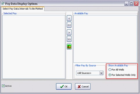
To display pay intervals, select the “Pay” option under the Picking Type Option then click the “Select Pay” button on the guide (highlighted in red).  This opens the Pay Data Display Options screen.

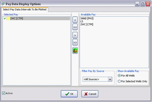
This screen shows pay zones already in the project, and can be filtered to show either pay intervals for the selected wells in the Log correlation Tool or to show the pay intervals for all wells in the project.  These pay intervals can also be filtered by the source.

In the example below, notice that the option for showing pay “For Selected Wells Only” (highlighted in red) is turned on.  Since none of the selected wells have any pay selected, nothing appears in the “Available Pay” window.

In this example, a 2nd Wall Creek pay interval already exists in the database.   Changing “For Selected Wells Only” to “For All Wells” displays all the pay zones in the project.  Notice in the example below that there are pay intervals both for lithology (“LS” and “Sand”) as well as for actual reservoir pay (“2WC”).  To display a pay interval, select it on the Available Pay list and click the “<” button to bring it over to the Selected Pay list on the right. To enable editing on the pay zone, make sure to select the small checkbox to the left of the pay zone’s name.  A green check, like that shown in the example below, signifies that the pay interval can be edited.

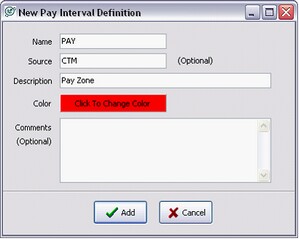
To create a new pay interval, select the button on the Pay Data Display Options window.  This brings up the New Pay Interval Definition box.  Enter the name, source, description, and color of your pay zone.  Select “Add” to add the pay interval to Petra’s database.

Step 7 – Picking Pay Intervals

Selecting “Pay” on step 5 changes the Quick List to show the Pay Intervals toolbar.

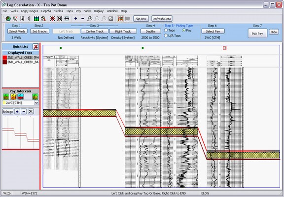
Begin Picking:   After selecting the appropriate pay interval, left click once in the appropriate location on the wellbore to create the top of the pay interval, and again to create the bottom.  To continue picking wells across your cross-section, simply click on the appropriate depth on other wells.  Petra will draw a hatched box covering the interval, as shown in the example below.  This hatching indicates that the pay intervals are not saved to the database.  When finished, right click the mouse button.

This brings up the option of saving the new pay intervals to Petra’s database. Selecting “No” will erase all unsaved pay picks.  In other words, if you make 25 correct pay picks in a row followed by a single bad one, make sure to select “Yes” and go back to fix the bad pick.  Selecting “No” will erase all the unsaved good picks as well as the single unsaved bad one.

Once saved, the hatched lines on the pay intervals disappear to signify that the pay intervals are stored to Petra’s database, as shown in the example below.

Move Picks:  To move pay picks, select this button.  Left click the top or bottom of a pay interval and drag it to the new location.  The pay interval will be hatched to show that the changes haven’t been saved to the database.  When finished, right click the mouse button.  This brings up the option of saving the new pay intervals to Petra’s database. Selecting “No” will leave all unsaved pay picks unchanged.

Delete Picks:  To delete picks, select this button and left click inside the pay interval.  When finished, right click the mouse button.  This brings up the option of saving the new pay intervals to Petra’s database. Selecting “No” will cancel all unsaved pay deletions, leaving the pay picks unchanged.

Create New Interval Name:   This brings up the New Pay Interval Definition screen.  Enter the name, source, description, and color of your pay zone.

Picking Faults

The Log Correlation Tool can show faults and fault gaps that represent missing section.  Fault intervals are stored to Petra’s database, and are shared among different modules and different users.

Step 6 – Picking Faults

To display pay intervals, select the “Fault” option under the Picking Type Option then click the “Pick Fault” button on the guide (highlighted in red).

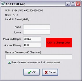
This changes the cursor to a crosshair.  To create a new fault, click on the intersection of the fault with the depth track.  A single click brings up the “Add Fault Gap” screen.  Note that clicking and dragging the cursor up and down will calculate and automatically calculate the missing section for the fault. It’s not necessary to fill in a name, source, or comment for every fault, but doing so can help distinguish between different interpreters’ work.

Fault gaps can be shown in a stratigraphic cross section and help to account for missing section.  To add fault gaps, select Faults>Display Options and select “Fill Fault Intervals.”   Note that you can limit faults by a source name, which can be useful in large multi-user projects.

To delete a fault, select the “Delete Fault” button and select the fault to delete.  This will delete the fault throughout the entire project, so be careful not to erase another interpreter’s work.  On a stratigraphic cross-section with fault gaps, make sure to click on the top of a fault gap to delete it.

Making another Cross-Section.

After you pick your first set of tops and pay, it’s not necessary to go through the entire process again for a new cross-section.  Petra saves column settings, default logs, depths, and top information to apply to your next set of wells.  To make a new cross section, all you’ll have to do is select the new set of wells (Step 1) and make adjustments in the default and/or assigned raster logs (Step 3).  Continually making small improvements to your default Log Type list as you make new cross sections is a good use of your time – the better and more comprehensive your default Log Type list, the less time you have to spend individually assigning raster logs to wells.

Other Display Options

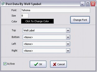
Plotting Well Data around Well Symbol – To plot well data around the well symbol at the top of the screen, select Wells>Plot Data around Well Symbol.  This brings up the Post Data By Well Symbol screen.  Here you can select which well identification data will be plotted around the well symbol.   In the example below, the wells’ label is plotted above the well symbol.

Well Symbols - While in the Correlation Tool’s main screen, dragging the lower line of the frame containing the well symbols increases and decreases this space.  The  and  buttons on the toolbar at the top of the screen toggle the well symbol and well data on and off, respectively.

The example below shows well labels displayed over each well symbol.

Plotting Log Scale Information – The tops of raster images usually have scale information for each column.  If this scale information is calibrated, it can be shown on the Log Correlation Tool’s main screen. To show and hide this raster scale information, click the  and  buttons on the toolbar at the top of the screen.  The next step is to tell Petra how the scale information is stored in the raster calibration.  Under Logs/Images>Log Header Display on the menu bar at the top of the screen, select “Header”, “Lower Scale”, or “Upper Scale.”   Many older Petra projects store scale information as the “header.”  Once this data is displayed, dragging the lower line of the frame containing the scales stretches and squeezes the image scales for readability.

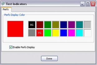
Test Indicators  - Select Wells>Plot Test Indicators to bring up the Test Indicators screen.  Select the display color for perfs, and click “Enable Perfs Display.”  The Log Correlation Tool will display perfs as a colored box on the depth track.  The example below shows perf indicators as a red rectangle on the depth track (highlighted in green).

Zoom and Scroll

For detail work, it’s probably advantageous to zoom and scroll on the cross section.  There are two ways to zoom in and out on the Log Correlation cross section.

Toolbar Zoom – The toolbar has a set of zooming tools: .

“+” and “-“ zoom in and out by 1/2 onto the center of the screen.  The button allows you draw an area to zoom.  The  button returns to the last zoom setting, while the  magnifying glass removes all zoom to return you to the default scaling.

The Pan and Scroll Window - This window on the Quick List log correlation window pans and scrolls around a zoomed cross-section.  The “enlarge button” creates an additional window, which is useful for double monitor setups.

Like the toolbar zoom, the “+” and “-“ zoom in and out of the center of the screen, while the “X” removes all zoom.  The extents of the log correlation main window are shown in red on this window. Dragging this red outline scrolls the extents of the main correlation window at the current zoom level.

Scrolling with the Arrow Keys Window – When zoomed in on a section, you can also quickly pan across the section using the arrow keys.  By default, the screen will pan by 50% of the currently displayed screen with every key press.  To change this scrolling percentage, go to Display>Arrow Keys.

Smooth Scrolling with the Alt Key – When zoomed in on a section, you can smoothly move the section by pressing and holding the Alt key.  Clicking and dragging any point on the zoomed in screen will then move the shown part of the cross-section.

The Right Mouse Button

Many common commands and some context-specific commands are available by clicking the right mouse button on the cross section.  A familiarity with these commands can ultimately add up to huge savings in time and effort.

The right mouse button accesses several common commands related to tops.  Place your mouse over the top right click the mouse flatten on, hide, or null the closest picked fm top.  To start picking the selected top under the Pick Tops Quick List, right click and select “Start Picking Top(s).”

Slip Box

The slip box takes a screenshot of a part of the cross-section and places it into a separate window inside the cross-section.  This section of the log can be a great help to correlation between one log and another.  The slip box window can be moved around the screen, as well as stretched and squeezed.  The slider box on the top of the window changes the box’s opacity to make it easier to overlay on top of other logs.

Shifting Wells Up and Down

Logs can be shifted up and down to facilitate correlation.  Press Shift and click the well to move the entire log up and down relative to the other logs.  To undo any shifting, select the “Refresh Data” button on the toolbar at the top of the screen.