|
This transformation applies a few different filters to a selected log curve, including a smoothing filter, a square wave (or box) filter, and a derivative filter. This tool can apply any combination of the three filters. When multiple filters are selected, Petra will apply them in the order they are listed from top to bottom. This log transformation is available on the Advanced Transforms tool.
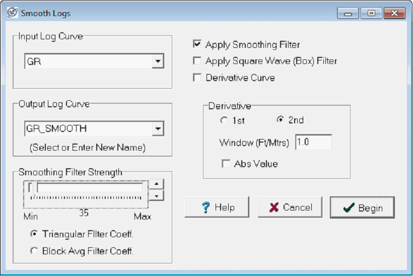
Input Log Curve This dropdown menu selects the desired input log. In the example above, the GR curve is selected.
Output Log Curve This dropdown/entry field selects the name of the copied log, which can be either an existing log or a new log name. Its usually a good idea to either make a backup of the original curve or to filter only a copy of the original data. Note that selecting a pre-existing log will overwrite the curve. In the example above, the output log will be written to GR_SMOOTH.
Smoothing Filter
The smoothing filter is a rolling average that tends to decrease small scale jitters in the curve. The filter itself is a rolling average, meaning that for every data point in the curve Petra examines a number of points above and below. A five-point rolling average, for example averages the 2 points before the data point, the actual data point, and the two points after the data point. Petra can apply anywhere from a 3 point rolling average to a 999 point rolling average.
Apply Smoothing Filter - This check box actually applies the smoothing filter to the logs. Note that the smoothing filter can be applied in combination with the other filters.
Smoothing Filter Strength - This section controls the details of the smoothing filter. The Smoothing Filter Strength slider bar establishes the number of points used in the smoothing process: the minimum of 3 points translates to a relatively small smoothing effect, while the maximum of 999 points greatly smoothes the data probably unrecognizably so for most data sets.
Petra makes a distinction between Triangular and Block Average smoothing. A triangular filter is a weighted average, where points in the rolling average closer to the actual data point have more weight than points more distant from the data point. A Block Average filter, on the other hand, gives all data points all equal weight in the average regardless of its distance from the data point.
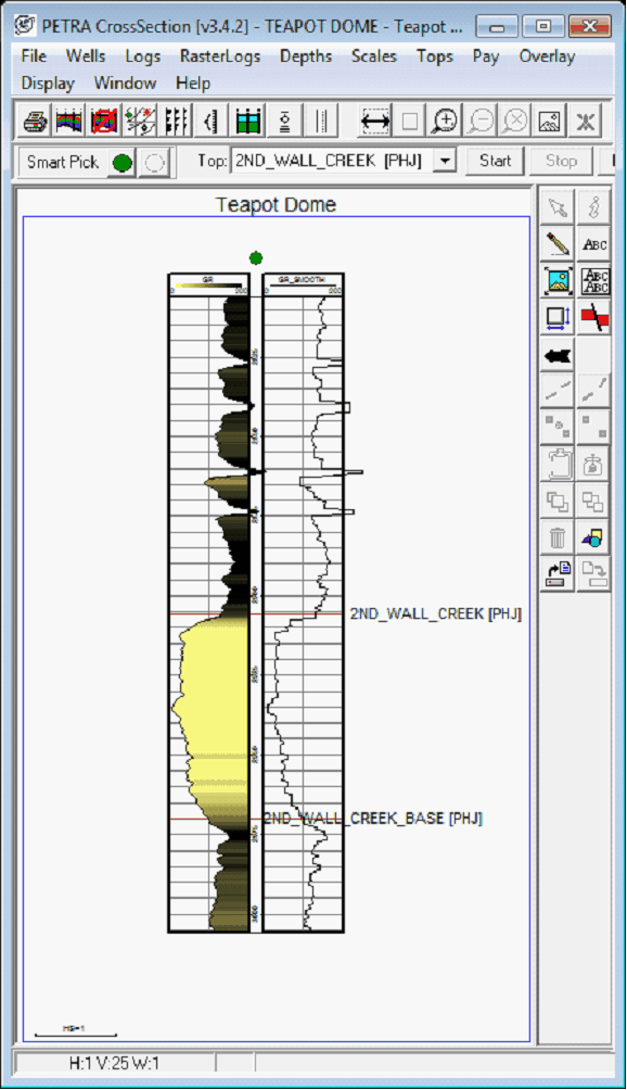
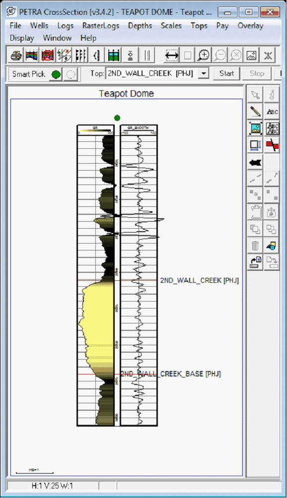
The example below shows a smoothing filter with a strength of 35 on the right relative to the original curve on the left.

Square Wave (Box) Filter
The square wave filter looks for parts of the curve with rapid changes from high to low values, and replaces these with flat, boxy interfaces.
Apply Square Wave (Box) Filter This checkbox actually applies the square wave filter to the data. Note that the square wave filter can be applied in combination with the other filters.
The example below shows the box filtered gamma curve next to the original curve on the left.
Derivative Curve
A derivative curve highlights the rate of change for a curve to highlight inflection points in the data; similarly, the second derivative calculates the rate of change of the derivative to further highlight the differences between inflection points.
Derivative Curve This checkbox actually applies the derivative filter to the data. Note that the derivative filter can be applied in combination with the other filters.
Derivative - This section controls the details of the derivative curve filter.
1st and 2nd - The 1st button calculates a 1st derivative of the input log, and the 2nd button calculates a 2nd derivative of the input log.
Window - This entry box sets the width of the derivative calculation; by default, Petra analyzes a 1 foot/meter window around any specific data point. Larger windows increase the effect of larger multi-foot transitions and decrease the influence of small scale changes in the curve.
Abs Value This button sets the derivative curve to only use positive values. By default, the derivative curve calculates positive values for positive changes in the 1st or 2nd derivative, and negative values for negative changes in the 1st or 2nd derivative.
The examples below show a 1st derivative curve relative to the original log on the left, and a 2nd derivative curve relative to the original log on the right.

|