Create Contour Grids (Directional Well Module)

Directional Well Model: Contours > Create Contour Grid

To create a contour grid:

• Open the menu item
• Click on the Create Contour Grid button on the icon bar.

Data tab

Method tab

The Method tab controls the grid size and surface style of the gridding.  The grid size of a grid largely controls how many points are in a calculated grid, which has a direct bearing on contour line smoothness and how well the computer-generated contour lines honor the data.The grid method, on the other hand controls how Petra interpolates the grid from one data point to another.

Grid Size

On a rectangular grid, the grid size determines the spacing between horizontal and vertical interpolated grid node values, as shown in the example below where the blue grid nodes are evenly spaced between a set of wells.  A grid spacing of 900 translates to grid nodes 900 apart both north-south and east-west.   Small spacing leads to more grid nodes, which generally honor the data better but require much more computer time.  Large spacing, on the other hand, tends to generate smoother contours with less computer time but at the cost of a less rigorous tie to data points.  The grid size section offers several methods for setting the grid size.

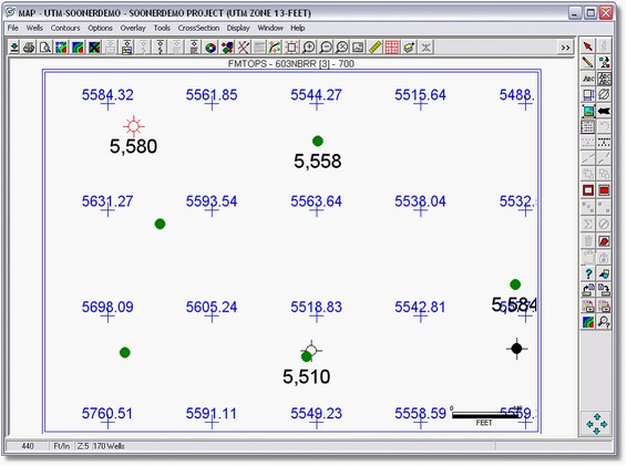
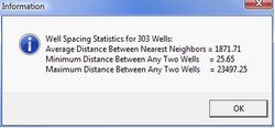
Use Grid Size of (XY units)This option sets grid spacing to a user-input X and X grid size in map units (feet or meters).  A good rule of thumb here is to use ½ the average well spacing.

To calculate average well spacing, select the Well Dist…button on the Data tab (highlighted below on the left).  The Well Dist… button on the gridding screen (on the right) gives statistical information on distances between wells, including average distances.  This tool will calculate distance statistics between all wells displayed on a map without discerning if they have data or not.  In other words, if you have a large number of closely spaced wells but only a few of those wells have data, this well distribution box will give you an average distance that is too small.

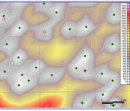
Compute Optimum Size From Z Data - During gridding, Petra will compute a grid size based on the well data distribution.

Set Rows and Columns Slider Bar – Instead of setting a specific grid size, this option instead sets the total number of horizontal and vertical rows for the grid.  Sliding the “Coarse to Fine” slider bar changes the number of rows and columns used in the grid.  Notice that as these are changed, the x and y grid spacing sizes change accordingly.

Match Grid Size of Grid This option sets the grid size of the new grid to exactly match the grid size of an old grid.  Select this option, and use the drop down menu to select the grid file to be matched. Note that the X and Y sizes are updated to show the grid sized used.

Mathematical calculations between two or more different grids require the size and spacing of each grid to match exactly.  As an example, creating a hydrocarbon pore volume grid (where HPV = thickness * porosity * hydrocarbon saturation) would require the isopach, porosity, and water saturation maps to all have the same grid spacing.  Using this option to match the porosity and hydrocarbon saturation grid size to the initial isopach grid will save considerable time later.

Surface Style

This option determines the shape and characteristics of the gridded surface by applying different mathematical functions to the original data. Surface styles interpolate the data between data points on both rectangular and triangular grids.

Highly Connected Features - This is Petra’s default gridding style.  It uses a least squares gridding algorithm that tends to preserve trends in the data and works well for most data, particularly structure maps and gently changing petrophysical data. The Highly Connected Features surface style works well with faulted reservoirs.  This surface style tends to not do well with rapidly changing or large contrasts between data points such as production in a closely-drilled field.

This method tends to avoid geologically unrealistic contours (or “artifacts”) on the edges of the grid, though contours can to be somewhat jagged and uneven with small grid sizes.  The application of surface flexing (“Smooth Contours Using Grid Flexing” immediately below the Surface Style drop down menu) works well with this surface style, as it tends to smooth and even out the spacing between contour lines.

Disconnected Features – This surface style uses a linear projection algorithm that tends to produce closed-off features.  This surface style can useful for mapping patch reefs or isolated channels.  The Disconnected Features surface style can be used with faults.  Contours generated from this surface style can be uneven and jagged, but this is easily remedied by adding surface flexing (“Smooth Contours Using Grid Flexing” immediately below the Surface Style drop down menu).

Since this method calculates grid values from a projected linear slope between one data point to the next, the Disconnected Features surface style is susceptible to a couple of different types of gridding artifacts.  At the edge of a map this surface style extends the nearest linear projection when calculating Z values, making it particularly prone to “runaway grid values” on the edge of the map.  The disconnected nature of the surface style also tends to make “bumpy” maps where two adjacent wells form an adjacent dome and a bowl instead of a more generalized trend.

Simple Weighting With Slopes – This surface style calculates a grid using three steps.  Petra first calculates a slope for each data point based on surrounding data points.  These slopes are then used to project the data points’ Z values out to each individual grid node.  Finally, this surface style takes the weighted average of the projected Z values.

The Distance Weighting Damping Factor on the Advanced tab can greatly affect this surface style.  This option uses any value from 1 to 8, with a recommended default setting of 2.  With a small factor, more distant data points have more influence on an individual data point which tends to average the grid node; this usually results in a smoother grid.  With a larger factor, close data points influence the individual grid much more than more distant data points.  The recommended value for this factor is 2.  For more information, see the help file on the Advanced tab.

Simple Weighting Without Slopes – This surface style applies a weighted average to the data points around each grid node.  In contrast to the Simple Weighting With Slopes surface style, no slope information is used. This option is useful for very dense control such as 3D seismic bin locations.

The Distance Weighting Damping Factor on the Advanced tab can greatly affect this surface style.  This option uses any value from 1 to 8, with a recommended default setting of 2.  With a small factor, more distant data points have more influence on an individual data point which tends to average the grid node; this usually results in a smoother grid.  With a larger factor, close data points influence the individual grid much more than more distant data points.  The recommended value for this factor is 2.  For more information, see the help file on the Advanced tab.

Distance Grid - This surface style calculates the distance to the nearest data point for every grid point.  Put another way, the grid right next to a data point will have a low Z value, while a grid a great distance from any data point will have a high Z value.  Contouring this distance grid can be a useful way of visualizing drainage and bypassed parts of the reservoir.  Parts of the grid with a high distance to the nearest well are less likely to be drained than parts of the grid with a low distance.

Again, this method only calculates distance to the nearest selected data point, which can include contour lines and control points in addition to wells.  If “Use Overlay Contour Lines” is selected on the Data tab, the surface style will calculate the distance from the nearest well or the nearest contour line.  This renders any visualization of drainage useless, so be sure to only select “Zone Data” for this surface style.

Closest Point - This option simply sets each grid node to the value of the closest data point. It doesn’t interpolate between data points, and is really more useful for resampling existing grids.  It is best used with very dense data such as 3D seismic coverage or with legacy XYZ grids.

Minimum Curvature Tension - This surface style attempts to create a very smooth, gradual surface.  Contour lines with this method are smooth and evenly spaced, which makes this style a good choice for gently changing petrophysical properties and simple structural settings.

This method cannot be used with faults.   Since the minimum curvature algorithm is also available under the “Smooth Contours Using Grid Flexing” option (immediately below the Surface Style drop down menu), so you can use the Highly Connected surface style (which works well with faults) along with the grid flexing option.  Since this method strives to have as simple a surface as possible (one with a “minimum curvature”), this surface style tends to smooth over some of the variation in data points.  In short, this method has the potential to “not honor the data” as well as other methods.  Edge effects with “runaway Z values” are also common with this method.

The "Min Curvature Tension" setting below can greatly affect this surface style.  Practically, high tension grids – particularly above 5 - have smoother and more even contours but may not honor the original data as well as lower tension grids.

Flex Grid Factor – Flex Grid Factor adds an additional step after gridding to generate smoother, more even contour lines.  When this option is selected, Petra first uses the selected surface style to interpolate between the data points to create grid nodes.  Next, Petra applies the minimum curvature surface style to both the original data points and to a decimated sample of the newly-interpolated grid values.  This option can be set anywhere between 0 and 12.  Setting a low grid factor will keep a relatively strong primary surface style, while a high grid factor will increase the relative strength of the minimum curvature surface style.

Grid flexing is also influenced by the “Min Curvature Tension” option on the Advanced tab.  Practically, high tension grids – particularly above 5 - have smoother and more even contours but may not honor the original data as well as lower tension grids.This option changes the relative strength of the “Smooth Contours using Grid Flexing” option.  Low Grid Flex Factor create final grids that  look like the original surface style, while higher Grid Flex Factors will create a grid that looks more like a Minimum Curvature grid.

Min Curvature Tension - Setting this option Petra first interpolates the data points with the selected surface style, then adds an additional step to interpolate both the original data points and the newly created grid values with the minimum curvature gridding algorithm.

Mathematically, this option controls the decimation of the initial grid, and can be set from 2 to 12.  When this option is set to 2, every other original grid point will be used in the Minimum Curvature step.  In this case, a large number of initial grid points remain which constrains much further interpolation from the second minimum curvature interpolation.  When this option is set to 12, only every 12th original grid point will remain.  The relative low number of initial grid points allows for more interpolation from the Minimum Curvature step.  In short, the lower the Grid Flex Factor, the more the final grid will look like the original surface style.  Higher Grid Flex Factors will create a grid that looks more like a Minimum Curvature grid.

Advanced tab

Max Pts Per Octant – Petra interpolates the value of each grid node from surrounding data points.  This option sets the maximum number of data points in each octant used for each grid node, and can be anywhere from 1 to 8.  For example, with a value of 2 the gridding process will use a maximum of 16 data points (2 for each octant) distributed around the grid node.

When determining which data points will be used for each grid node, Petra first divides the area around the grid node into eight wedges, or “octants.”  Petra then uses the closest data points (up to the maximum set by this option) in each octant for calculating an individual grid node’s value.  Dividing the surrounding data into octants helps avoid grid nodes that are too heavily biased by data points in one direction.

Max points per octant set to 1 (left) and 2 (right)

Use Natural Neighbors – This option causes most surface styles to use a “natural neighbors” triangulation search instead of the normal octant search when selecting data points to interpolate for each grid node. This tends to provide a more localized interpolation, which can benefit grids with dense data point coverage.  Since this adds an additional pre-gridding triangulation stop, this option can increase gridding time.

When deciding which data points to use for each grid node, most rectangular grids styles (Highly Connected Features, Disconnected features, Simple Weighting With/Without Slopes) use an octant search where the area around a grid node is divided into eight wedges, or “octants.”  This octant search ensures that data points used for the grid point interpolation are evenly geographically distributed.  A natural neighbors search, in contrast, selects surrounding data points that can be connected by a triangular network. This option just changes how Petra selects the data points for interpolation, so the output will be a normal rectangular grid.

Octant search selects data points in 8 wedges around the node, while a natural neighbors search uses a triangular grid

Skip Well if Quality Code Contains – This option skips data points from wells that have specified quality codes.  Here, enter one or more values separated by a semicolon to indicate wells that are NOT to be used for gridding.

Tops tab

Skip Well if Quality Code Contains – This option skips repeat formation tops from wells that have specified quality codes.  Here, enter one or more values separated by a semicolon to indicate repeat tops that are NOT to be used for gridding.

Triangulation tab

The Triangulation tab sets changes the gridding from rectangular to triangular gridding. Triangular grids always honor the data at the cost of sometimes unrealistic changes in slope or dip.  Refinement adds more interpolation inside these triangles, which smoothes these grids.  Interior angle clipping reduces grid artifacts caused by widely separated wells on the edge of the map.

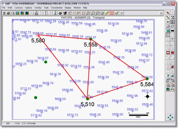
Instead of interpolating values for nodes at regularly spaced X and Y intervals, triangulation instead constructs a network of nearest neighbors using the data points.  Essentially, Petra calculates node values along lines (shown with lines) between data points.  These nodes form triangles known as “Delaunay triangles.”  Notice also that there is a node value directly on top of each well.  The resulting contours “honor the data” better because they are drawn using the actual values as opposed to interpolated data in rectangular gridding.  Triangular grids are better suited to closely spaced, or highly-variable data rather than widely separated data.

Check the Triangulate box to perform triangulation instead of rectangular gridding.

Triangle Refinement –   In a simple triangular grid, each Delaunay triangle is independent from every other triangle so calculated gradients on one triangle can differ significantly from an adjacent triangle.  This can lead to rapidly changing, geologically unrealistic dips and angular contour lines.  Contours from these simple triangular grids can look strange and can even cross.

Petra smoothes these triangular contours with a process called “triangle refinement.”  Refinement adds more points inside a Delaunay triangle to smooth the grid’s surface and contour lines.  These points inside the triangle are interpolated using Petra’s surface style (such as “Highly Connected Features”). selected on the Method tab and surrounding data points.  The refinement value selected here determines the number of additional points, which in turn governs the smoothness of the contours.  A refinement of 1 simply uses the existing data points with no interpolation, while a refinement of 16 adds a great deal of interpolated points inside each triangle.  Practically, a highly refined grid will have smoother contour lines than a grid with lower or no refinement.

Interior Angle – Triangular grids attempt to connect all data points together regardless of how far apart they are. The part of the grid based on an interpolation between distant data points often shows geologically unrealistic contours – especially on the edge of the map.  On the right side of the example below, two highlighted triangles have high interior angles of 172 and 160 degrees.  The area of the grid represented by these two triangles probably interpolates the data too far and should be removed.

The triangular grid between these distant wells has one corner with a large angle.  Filtering out triangles with this high interior angle helps to trim out overly-interpolated or geologically unrealistic parts of the grid on the edge of the map.  Setting the value here to 150, as in the example below, will eliminate all triangles with an internal angle above 150 degrees.  The smaller the angle, more edge triangles are removed. Suggested values are 120 to 160 degrees.

Fast Local Slope Interpolation Method –Normal refinement uses the selected surface style to interpolate data points inside each Delaunay triangle based on the surrounding “neighborhood” of data points.  The “Fast Local Slope” method instead uses partial derivatives to interpolate inside each triangle.  In other words, while the normal refinement method attempts to make a more coherent regional picture based on outside data, this method simply uses only the data points in the Delaunay triangle.  Consequently, this method is quick, but is prone to geologically unreasonable dip changes and other artifacts.