How to Digitize a Raster Log |
|
Raster logs are scanned copies of paper logs saved as image files. Digital logs, on the other hand, store log values in a form that is directly readable by a computer. Digital logs have several advantages over raster logs: theyre more easily stored in Petras database, look great in a cross section, and can be calibrated and used in calculations. Converting a raster log into a digital log is called digitizing. Going from a simple image file to a digital log involves two major steps: depth calibrating the raster image, and tracing the desired log curve. This guide walks through depth calibrating and digitizing the GR curve on the D-122 well in the TUTORIAL project. Depth-Calibrating the Raster ImageRaster logs are scanned copies of paper logs saved as image files. Petra needs to know what part of the image corresponds to which depth in order to assign values during digitizing. Most commercial data vendors depth register their data, but images directly from scanners and state providers are not depth calibrated. The first step to calibrating a raster is to select the correct well in the Main Module. For this example, select the D-122 well in the Main Module.
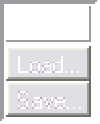
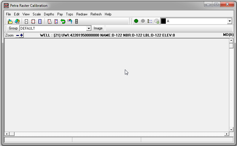
The Raster Calibration ScreenTo start calibrating a raster log, open the raster calibration screen. In the Main Module, click on the Assign/Calibrate button on the Rasters tab. This opens the Calibrate Log Image screen. Notice that the selected wells UWI and name appear on the screen.
Next, open an image file by going to File>Open Image on the menu bar. Navigate to the specific image file and select it. By default, the D-122s raster log will be located here C:\geoplus1\Projects\TUTORIAL\IMAGES\D-122.TIF. It might be useful to use the zoom buttons (
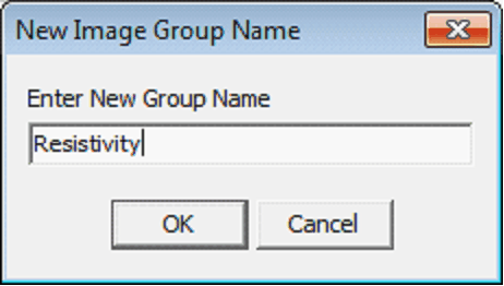
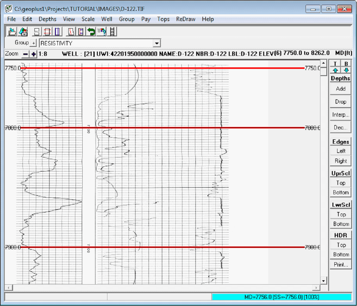
Group NamesAll raster images are assigned group names. A group name usually describes the log type (like Resistivity) and/or scaling (1, 2, or 5) of a log image. Select the appropriate image group from the "Image Group Name" drop-down list. To add a new group, click the + button next to the group names dropdown box (highlighted in red in the example below) or to Group>Add or Delete Groups... on the menu bar. Since the raster image is a resistivity log, add a Resistivity group.
When selecting or creating group names, its generally better to aim for fewer, more general group names rather than create many precise group names. The more group names in a project, the tougher it will be to display cross-sections later. Though most of the tools to calibrate logs are available from the menu bar at the top of the screen, the quickest and easiest way calibrate a raster log is to use the Depth Calibration Toolbar (highlighted in blue in the example above). To turn on this toolbar, go to View>Depth Calibration Toolbar on the menu bar. Define the Calibration Depths
To create a new calibration depth, click the Add button on the Calibration Tool Bar Alternatively, go to Edit>Add Depth Point on the menu bar. Next, position the horizontal cursor at the depth you wish to pick and click the left mouse button. You will be prompted for the depth value. After entering the depth value, the screen will redraw showing the new calibration depth point. Repeat the process for each new depth calibration point.
To change the location of the depth, click and drag the depth calibration point using the left mouse button. To edit the value of an existing depth, click on the depth calibration point with the right mouse button and enter a new value. The better the quality of the raster log, the fewer points necessary to depth calibrate the image. Most raster logs only really need a handful of points. Petra also automatically scales and places reference black lines every 100. Unlike normal red calibration lines, these cannot be moved they just show Petras scaling between your calibration lines. If these black lines look close to the actual image, your calibration points are sufficient. If the thin black calibration lines are off of the depths printed on the raster log, add new points or adjust your existing depth calibration points. Deleting Calibration Depths
You can also delete all depth calibration points by going to Edit>Delete All Depths... on the menu bar. Interpolating Depths
After creating two or more depth calibration points, click the Interp button on the Depth Calibration Toolbar or go to Edit>Interpolate Depths on the menu bar. Select the interpolation increment, and Petra will compute depths at your specified interval between the top and bottom depth calibration point. Saving CalibrationsThough its not strictly necessary for digitizing, this is a good point to save the calibration. A calibration file stores information like depth calibration points and edges, raster image file name, and group name. Saving a calibration file also updates the Petra database to link the image and group name with the currently selected well. Click the Save Calibration As
button at the top of the screen:
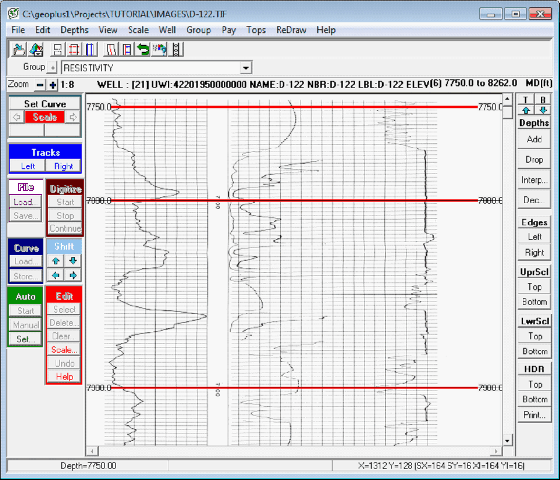
After saving the file, the group name will now show up on the Rasters tab in the Main Module, and you will be able to plot the raster in a cross section. Digitizing the CurveTurn On the Curve Digitizing ToolbarOnce the raster image is open, select View>Curve DigitizingToolbar on the menu bar at the top of the screen to toggle the toolbar on and off. It will appear on the right side of the screen.
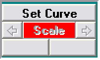
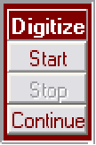
Select the Digital Log Curve and ScaleThe next step is to tell Petra the curve name and the scale for the log to digitize. Select the red Set Curve button at the top of the digitizing tool bar.
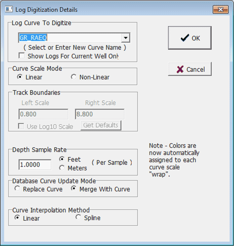
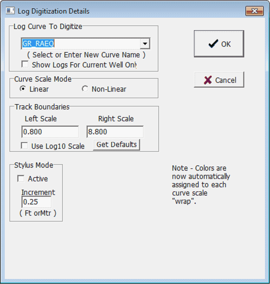
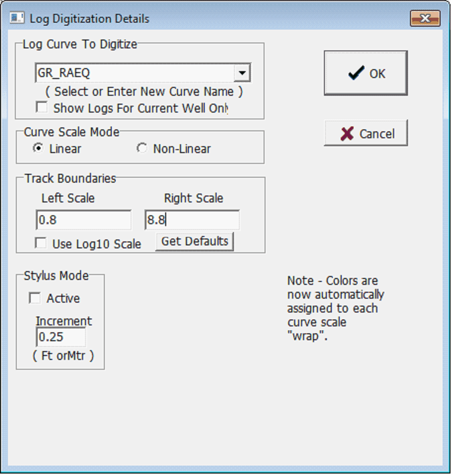
This button opens up the Log Digitization Details window. In the Log Curve to Digitize dropdown box, select an existing curve or enter a new curve name. This curve name will be the name of your digital log, so be careful about replacing an existing digital log for the selected well. Next, specify the curve values for the left and right sides of the track boundary. For curves on a logarithmic scale, such as resistivity, make sure to select the Use Log10 Scale button. For this example, well digitize the gamma ray curve. Notice that the footer of the D-122 log states that the GR curve is has a micrograms radium-equivalent/ton scale from a 0.8 to 8.8. In order to distinguish it from a more traditional gamma curve, it is named GR_RAEQ. The track boundaries are set below just like on the footer, the scales go from 0.8 to 8.8. The actual raster log wraps when the count exceeds that 8.8, but thats easy to deal with later.
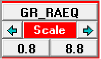
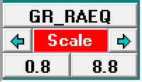
Notice that the same scale box on the digitizing toolbar now shows the name of the curve to be digitized and the scale.
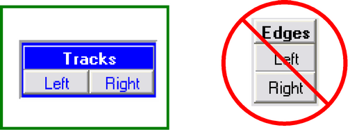
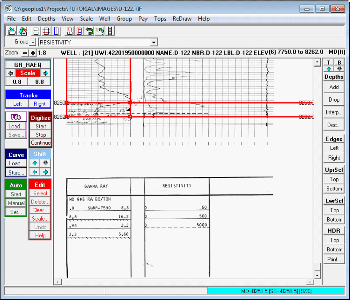
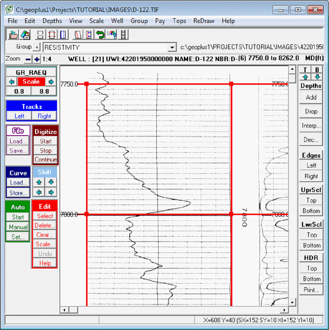
Set the Left and Right Track EdgeThe next step is to set the left and right edges of the track containing the curve to be digitized. Petra uses these lines to calculate a numerical value for the digital log. Notice that the footer of the log states that the curves scale is from 0.8 to 8.8. The left and right digitizing track edges will tell Petra where 0.8 and 8.8 are, with digitized points in the middle scaled accordingly. As an example, a digitized point halfway between the left and right track edges will be stored as 4.8. To set digitizing tracks, select the Left and Right buttons in the Tracks box on the digitizing toolbar and then click on the respective track boundary. Remember that digitizing tracks (in the blue box on the left side of the screen) are different than track edges.
In the example below, the left and right digitizing track edges (in red) are around the first track containing the gamma ray curve.
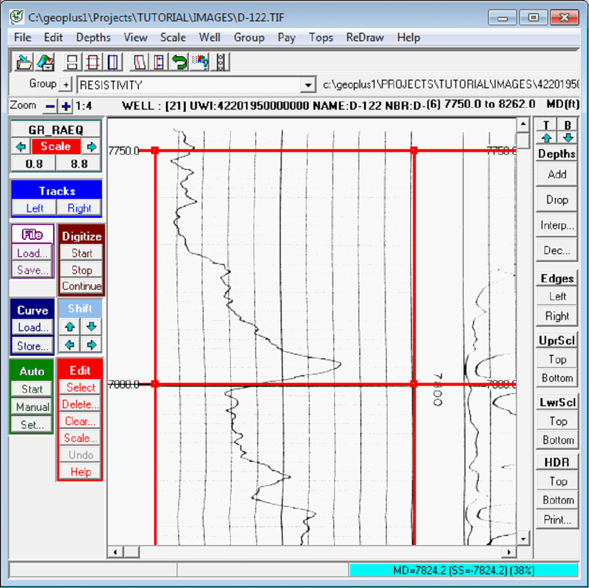
Raster logs are often curved due to paper stretching or slipping during scanning. Crooked logs mean inaccurate digital logs. To handle crooked rasters, you can either straighten the whole image, or adjust the left and right track boundaries. Straightening the whole image has two advantages. You only have to adjust one track straight edge instead of two separate track boundaries, and you can save your work as a new copy of the straightened raster image. If youre digitizing multiple tracks on the same raster log or a fairly long section, straightening the whole image will ultimately save time. For information on how to straighten a raster log, see here. The other way of dealing with crooked raster logs is to adjust the left and right digitizing track lines. Both the left and right track edges have control nodes at every calibration depth. You can move these control points with the left mouse button to align track edges with the image. The advantage to this method is that it saves a step and eliminates the need to store multiple copies of the raster image. Simply adjusting track boundaries is easier for short digitizing runs on straight raster images. Draw the Digitizing LineThe next step is to actually trace the log curve with a digitizing line. As mentioned above, Petra reads these lines and compares them to the track boundaries in order to calculate a digital log value for each depth. There are two major ways to draw these lines: Manual and Automatic. Draw the Digitizing Line - ManualTo manually digitize log curves, first click the Start button on the Digitize section of the digitizing toolbar.
The Log Digitization Details box will reappear to confirm the settings on the log and scale. Here, you can also select the digitizing style. The default drawing style is that every left click creates one control point on a digitizing line. You can also select Stylus Mode, which continually records points at the specified increment when you hold down the left mouse button. In the example below, the stylus mode will create a point every half foot. Select OK to keep the log settings and the pick mode and return to the raster image.
The next step is to draw the digitizing line. In stylus mode, click and hold the left mouse button to continually record points. If using point and click mode, simply click on top of the curve to create points and draw a line. If in point and click mode, you can temporarily activate the stylus mode by holding down the ALT key. Notice that on the bottom of the screen Petra shows the depth and the value of the curve at the mouse position. These are the values going into the digital log, so its a good idea to check this in the beginning to make sure the curve and depth values are reasonable.
To stop tracing the digitizing line, click the Stop button on the Digitize section of the toolbar or right click the mouse. Digitizing lines are divided into independent segments. Each time you select Start during manual digitizing, Petra brings up the Log Digitization screen and you create a new curve segment with its own scale. Selecting Continue, on the other hand, just adds more points to the existing curve segment at the same scale. You can have as many or as few curve segments as you want. For more on curve segments, see Editing Curve Segments below. IF YOU MAKE A MISTAKE, you can either immediately stop and fix the mistake or wait until the end. To fix a mistake you can either individually select and move control points (see Editing Curve Segments below), or simply select Continue and draw over the mistake. Draw the Digitizing Line - AutomaticPetra can also automatically follow and trace simple, bold, well-defined curves.
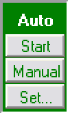
First, select the "Start" button under the "Auto" section, then click on the uppermost point on the curve to be digitized. The auto tracer will attempt to follow the densest portion of the log beginning at the selected point. You can press the ESC key or click the left mouse button to stop the auto tracer. The "Manual" button allows you to manually re-digitize over section not properly handled by the auto tracer. The "Set" button displays a screen for setting properties controlling the auto tracer.
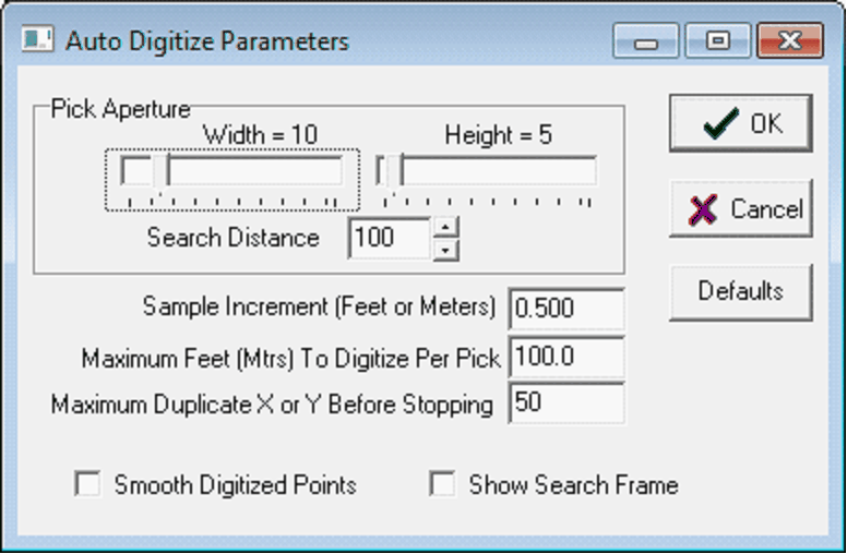
Pick Aperture - When automatically digitizing a curve, Petra looks for the darkest adjacent point within a window or aperture. The pick aperture sets the size of this window, which is by default 10 pixels wide by 5 pixels tall. Sample Increment This determines how many nodes will be created for a given foot of log. In the example below, the increment is set for 0.5, so one point will be created at every half foot. Note that this increment just determines the how smooth the traced line will be. The sample rate of the digital curve is independent of this number. Maximum Feet (Mtrs) To Digitize per Pick - This option sets the maximum distance Petra will digitize a line. Limiting line length prevents Petra from getting stuck on the wrong line and creating a large mess. Maximum Duplicate X or Y before Stopping - If Petra starts tracing a straight line, odds are good that Petra is following either a horizontal or vertical grid line. This sets the maximum number of duplicate pixels Petra will allow before stopping. Image FilteringThere are a few tricks that can help with auto digitizing. Since the tracing algorithm looks for adjacent dark pixels, it can easily get confused by vertical scale lines and horizontal depth lines. Petra can filter out straight horizontal and vertical lines. This process modifies your image file, so be sure not to save over the original image file and have a backup. Both of these filters can reduce the clarity of the curves as well, especially where the curves intersect the filtered horizontal or vertical lines. To restore the filtered lines select File>Reload Original Image.
Edit>Filter>Remove Vertical Lines
Edit>Filter>Remove Horizontal Lines
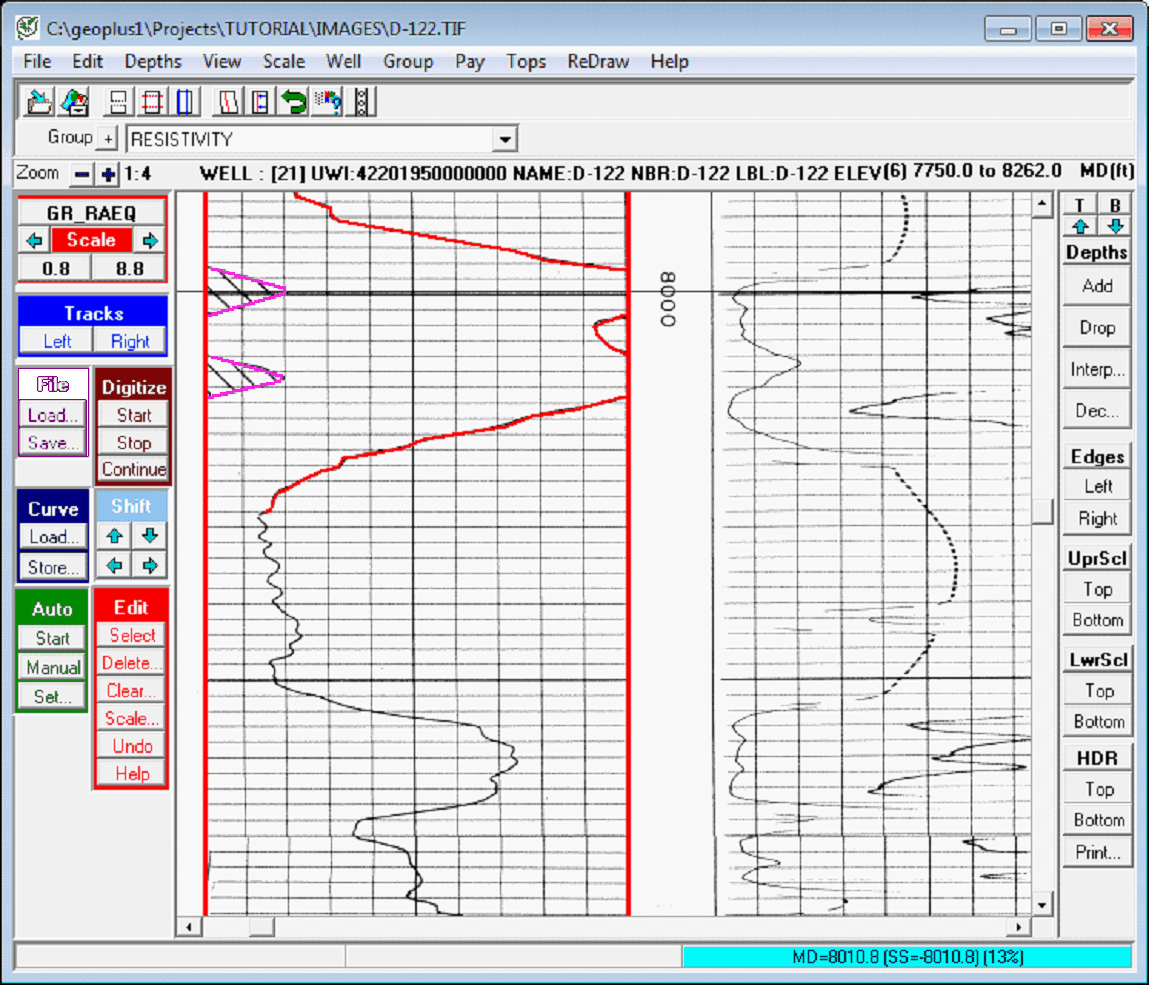
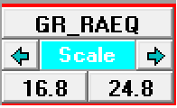
Changing the Track Scales (Curve Wrapping)Whenever the curve on the raster image reaches a track edge, the scale will "wrap" and the curve will reappear on the opposite side of the track. At this point, you will need to stop digitizing and change the scale. The left and right side track scale is displayed near the top of the Digitize Toolbar. Each curve scale range is displayed in a different color beginning with red for the base scale. There are 6 colors defined above and below the base scale. To increase the scale range and wrap the curve, click on either the
In the example below, the GR curve has started reading above 8.8, and has wrapped around the scale. At this point, right-click or select Stop.
Next, click the
Right click or select Stop to stop digitizing. Click the
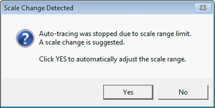
Scale wrapping also works for the automatic tracer. When it detects that the curve has run into the track edge, it will ask if you want it to automatically adjust the curve scale. In the example below, the automatic digitizer has spotted the track edge. Selecting Yes will stop the digitizer and automatically wrap the scale for you. The next step is to click on the uppermost part of the wrapped curve.
Editing a Curve Segment
Selecting a Curve Segment - To edit a curve segment, first click the Select button on the red Edit toolbar. Alternatively, double-click on the curve segment. Selecting a line segment shows each of the control points as small rectangles. To deselect a segment, click the right mouse button. In the example below, there are two curve segments. The top segment is selected, which shows all the control points for that line.
Changing Curve Scale Range - To change a curve segments scale range, first set the correct scale range at the top of the digitizing toolbar. Next, select the segment and click the "Scale" button. The curve section will then be set to the scale shown on the top of the scale bar. Breaking a Curve Segment - You can break a segment into two segments. First, select the segment. Then, hold down the CTRL-key and click on a segment control point. All points ABOVE the picked point will become unselected. They are now part of a different segment. Breaking and Deleting Part of a Segment - You can also break a segment into two segments then delete the bottom portion. First, select the segment. Then, hold down the CTRL and ALT-keys together and click on a segment control point. All points BELOW the picked point will be deleted. Using the Delete Rectangle - You can draw a rectangle to delete intermediate points of the selected curve segment. First, select a curve segment. Next, hold down the SHIFT-key and click and drag to form a rectangle. All points within the depth range of the rectangle will be deleted. The segment will be de-selected and two new segments will be formed. Deleting ALL Curve Segments - Click on the "Clear" tool bar button in the Edit section to delete all curve segments. Bulk Shifting a Curve Segment - Sometimes its useful to shift an entire curve segment. To move an entire curve segment at one time, first select the segment. Next, select one of the arrow buttons in the Shift toolbar. This moves the entire segment in the direction of the arrow. Saving and Loading Your Work-In-Progress
Store a Curve to the DatabaseThe final step of digitizing a raster log is to store the traced line as a digital log. In this step, the curve segments are resampled to the specified sample rate and merged together. When segments overlap in depth, earlier segments are replaced by later ones. In other words, where lines overlap, Petra will use the last drawn line. Once stored, the digital curve is available in Petras database for drawing in cross sections or calculations.
To store a curve, select the Store button on the blue Curve toolbar. This brings up the Log Digitization Details box. First, select the digital curve name you want the curve stored as. In the example below, well stick with GR_RAEQ. Notice that the options under Track boundaries are greyed out since each segment stores its own scale, theres no need to change this. Next, set the depth sample rate, which just sets how many samples will be stored per unit of depth. The default is 1 foot, as shown in the example below. If youll be using this log for calculations with other logs, make sure that this number matches the sample rate of your other digital logs. Most digital logs are stored on a half foot sample rate. Next, set the Database Curve Update Mode. If theres already a curve stored with the same curve name, this determines how the digitized log will be stored. Replace Curve will completely erase the old digital log and replace it with the new digitized curve. Merge With Curve will keep the old log and only replace the sections youve digitized. Finally, set the curve interpolation method. The linear method draws a straight line between control points, while a spline attempts to fit a curve between control points. The interpolation method on the main screen is linear, so most people digitizing already account for that when picking points. In other words, people mostly place the points close enough together for a linear interpolation to accurately trace the curve line.
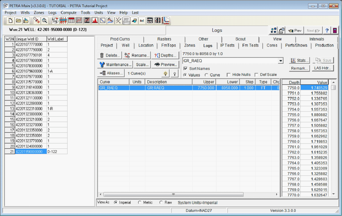
The now digitized log now appears in Petras database, and can be used for calculations or display. In the example below, notice how GR_RAEQ now has a value for every depth.
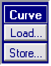
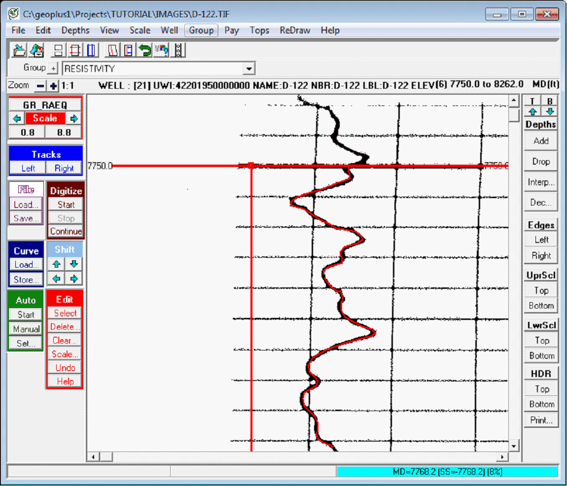
Loading a Curve from the DatabaseThe "Load" button under the "Curve" section lets you load a digital log curve from the database to display on top of a depth-registered raster curve. This is particularly useful for doing quality control on someone elses digitizing work.
First, set the left and right track scales. Next, select the red Scale button at the top of the digitizing tool bar.
Next, select the pre-existing digital log curve on the Log Curve to Digitize dropdown menu. This is the log youll load into the digitizing screen. Select OK.
Finally, select the Load button on the Curve toolbar. This will replace any digitizing lines on the main screen with the digital data from the selected curve in the database. Starting Another Curve If you want to digitize more than one curve, you will need to use the "Edit>Clear" button on the toolbar. This will remove previously digitized segments from memory so they don't get stored as part of the new curve. |

 ) on the upper right corner of the window to make the image larger or smaller.
 . Alternatively, go to
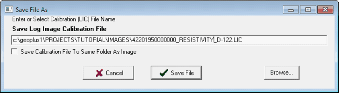
 button or on the right side scale value. To decrease the scale range and shift the scale to the left, click on either the
  button or on the left side scale value.
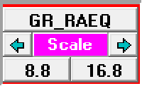

 arrow to wrap the digitizing scale to the right from 0.8-8.8 to 8.8-16.8 and select Continue to digitize the wrapped section of the curve. Note that the digitizing line skips a saddle in between the two hot highs; its perfectly reasonable to skip a section and come back to it later. Notice in the example below that the digitizing scale and the digitizing line are pink to show that they are on a 8.8-16.8 scale.
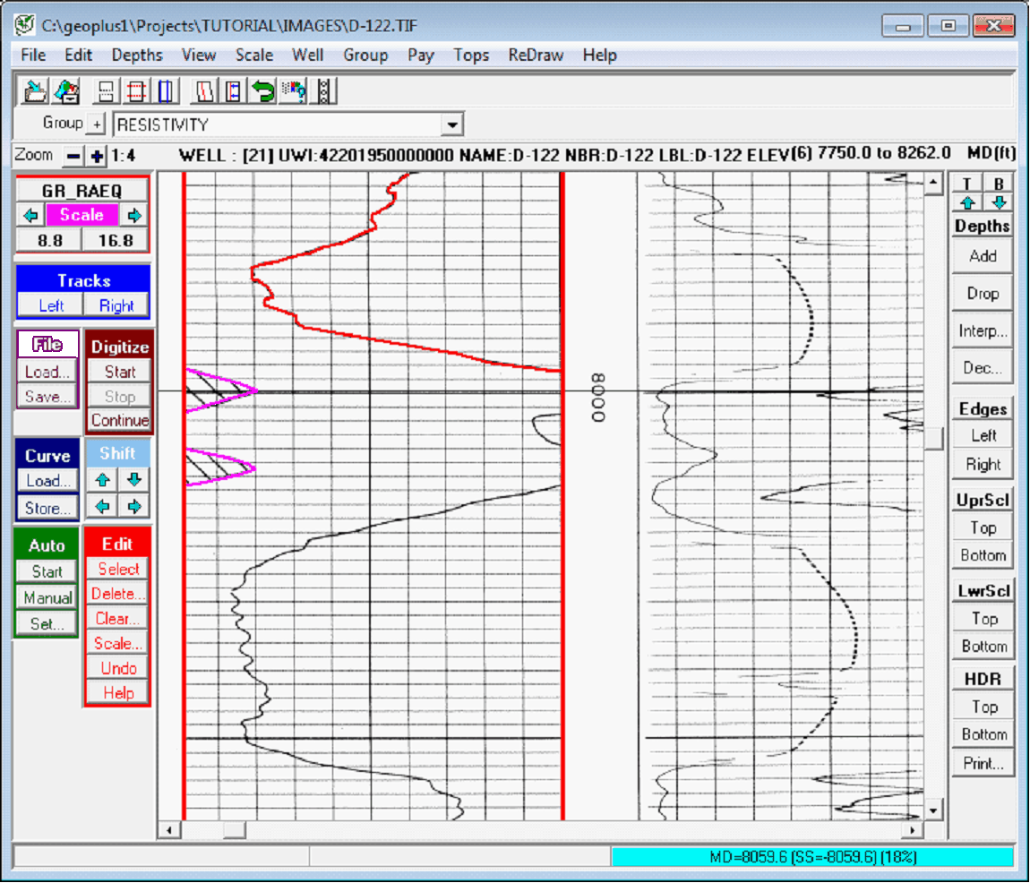
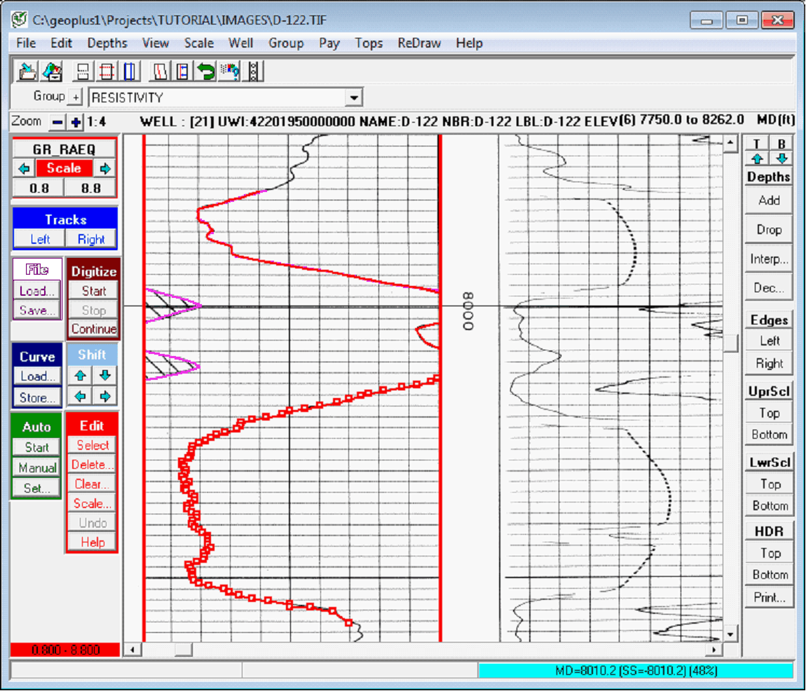
 button to wrap the scale back to 0.8-8.8 scale and select Continue. Notice that the digitizing line color has returned to red. Make sure to fill in the saddle in between the two high gamma count spikes.