Monte Carlo Simulation

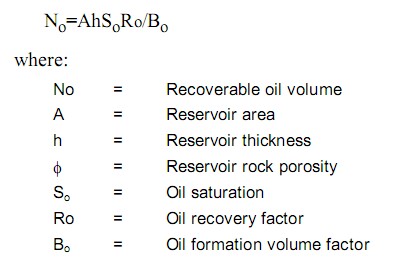
A Monte Carlo simulation calculates probability of recoverable gas in place using a range of inputs for variable volume, porosity, gas saturation, recovery factor, and gas formation volume factor.  The Monte Carlo Simulation is a standalone tool, and does not use any of the options entered on the Gas or Oil Volumetrics tab.  

Simulation Models

For oil reserve simulation, Petra uses the following model:

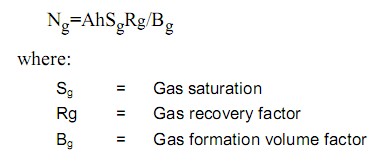
For gas reserve simulation, Petra uses the following model:

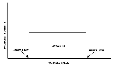
Reservoir Options

Volume – Enter the range of possible reservoir volumes in acre-ft.

Porosity – Enter the range of possible reservoir porosities.  Remember to use whole numbers instead of decimal percentages.

Gas Saturation – Enter the range of possible gas saturations.  Remember to use whole numbers instead of decimal percentages.

Recovery Factor – Enter the range of possible recovery factors.  Remember to use whole numbers instead of decimal percentages.

Gas Formation Volume Factor – Enter the range of possible gas formation volume factors in RB/MSCF.  

Reservoir Option Ranges and Probability

Each of the reservoir parameters can vary in a few different probability distributions.   For more detail on using probability distributions as well as strategies on estimating standard deviation, see the appendix at the end of this document.

Uniform – In a uniform distribution, all values between the minimum and maximum vales are equally likely. To use a uniform distribution, simply enter the minimum and maximum values.  

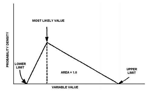
A Uniform Distribution

Triangular – In a triangular distribution, the “most likely” value has the highest probability with a gradually decreasing probability towards the minimum and maximum.  To enter a triangular distribution, enter the minimum, maximum, and most likely values.  The most likely value will be treated with the highest probability, with a linearly decreasing occurrence of values towards the minimum and maximum values.

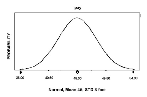
A Triangular Distribution

Normal - In a normal distribution, values are more probable around a single arithmetic mean, or average.  This creates a “bell curve” where values closer to the mean are more likely, where the standard deviation measures the average difference of the values from the mean.  To use a normal distribution, simply enter the mean and standard deviation

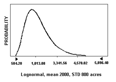
A Normal Distribution

Log-Normal – In a log-normal distribution, values are more probable around a single mean with an even distribution of the logarithms of surrounding values.  Log-normal distributions are common when there is multiplication of two or more normally distributed factors.  To use a log-normal distribution, simply enter the mean and standard deviation.

A Lognormal Distribution

Constant – A constant distribution actually has no variability at all and only contains a single value.  An example of a constant is the ultimate mortality rate, which is holding steady at 100%.

Monte Carlo Outputs

A Monte Carlos simulation generates many different possible reserves values, some of which are more likely to occur than others.  Petra displays these statistics in a few different ways on tabs next to the Monte Carlo tab.  

Report Output

The report output tabs shows recap of the initial reservoir parameters, a percentile breakdown of the simulation results (P10, P50, P90, mean reserves, and expected reserves), and a cumulative distribution table.  

The summary gives a brief statistical breakdown of the probability of different calculated reserves.  There is a 10% chance that the reservoir is equal to or less than the P10 value, a 50% chance the reservoir is equal to or less than the P50 value, and a 90% chance that the reservoir is less than the P90 value.  The mean reserves value is a simple average of all the calculated reserves values, while the expected reserves value instead weights results by probability.    

The cumulative distribution table expands the calculated percentiles to cover every 5%.   Each percentile gives the chance of the reservoir being equal to or less than the calculated reserves.  As an example, there is a 55% chance that the reservoir is equal to or less than the reserves value across from cumulative distribution of 55.

Probability Plot

This plot displays the probability density on the Y axis versus the range of possible reserves on the X axis.  Low reserves estimates on the left side of the graph are the result when everything goes wrong; this includes when the total volume, porosity, oil saturation, etc. are all on the lower end of the possible ranges.  Since the probability of all these different factors going wrong is low, the corresponding probability of these low end reserves is low.  The high side of the graph with large reserves, on the other hand is the result of everything going well, which also has a correspondingly low probability.  The bump in the middle of the graph corresponds to the highest probabilities; these are the outcomes of the more common reservoir parameters.

Cumulative Distribution Plot

This plot displays the cumulative probability on the Y axis versus the range of possible reserves on the X axis.  Each point on the line reflects the probability of the reservoir being equal to or less than the calculated reserves.  As an example, there is a 55% chance of the reservoir being equal to or less than the reserves value across from accumulative distribution of 55.