This transform uses log crossplot polygons to create new logs based on petrophysical criteria.  The Log Crossplot Module plots log curve values from the same depth together on a XY scatter plot or a ternary diagram.  Regions on this crossplot, when outlined by polygons, represent specific combinations of two or more logs.  Petra refers to these polygons as “facies.”  This transform creates a new log based on the crossplot facies; when the log data fits inside a polygon, the polygon’s facies value is stored to the log.  Facies logs can represent anything from pay flags to complete lithology descriptions.

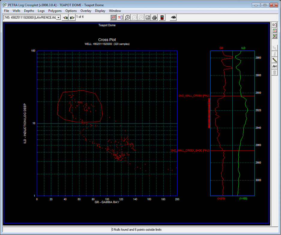
As an example, the crossplot below shows gamma and resistivity curves.  The polygon drawn on the log data represents the productive interval where gamma is lower than lower than about 90 API units and resistivity is above 10 ohmm.  The polygon outlining the region has a facies value of 1.  A facies curve transform applies this polygon to other wells.  The depths were the gamma and resistivity curves fall inside this polygon are assigned the polygon’s facies value of 1, and the parts of the well where the gamma and resistivity curves fall outside this polygon remain a null value.

This log transformation is available on the Advanced Transforms tool.

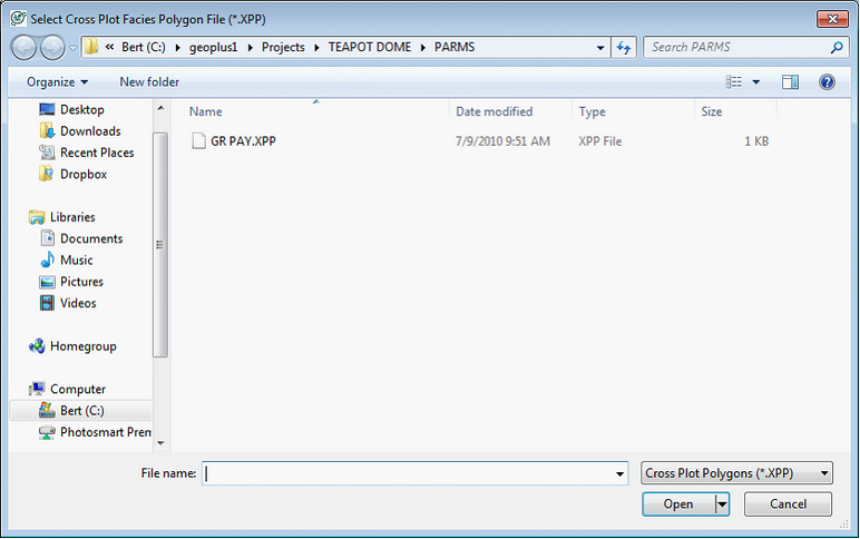
This transform requires a set of polygons.  These files are created in the cross plot module and have a *.XPP file extension.  When opening the Facies Transformation tool, Petra by default opens the current project’s PARMS directory.  Select the desired polygon file.  In the example below, the GR PAY.XPP file is selected.

Petra then opens the Facies Log from Cross Plot Polygons tool.  This tool is divided into several different tabs.

File tab

The File tab displays the selected polygon file, as well as the polygon file’s comments.  To change the selected polygon file, select the “Browse” button.  By default, facies polygon files are stored in the project parms directory.

Logs tab

The Logs tab sets the logs used in the facies curve calculation.  

X-, Y-, and Z-Axis – These dropdown menus change the logs used in the crossplot calculation.  By default, Petra will load the logs from the facies polygon.  Changing the logs will keep the polygon cutoff values the same.  In the example below, the GR and ILD curves are loaded in the X and Y axis.

Use Log Aliases – The transformation is picky about the exact curve name; if any of the X, Y, or Z logs are missing for a well, no output log is computed.  This option tells Petra to use log aliases during the transformation.  

Output Facies Log – This option his window also changes the name of the output facies curve; by default this is set to “FACIES” as in the example below.  To change the name, just enter in a new curve name.

Facies tab

The Facies tab sets the actual values used in the facies curve.  

Default Facies Value – This option sets the value assigned to the output log when the cross-plotted point does not fall in any of the polygons. Set a numeric value or enter the word NULL the use a null value for the default.  In the example below, it’s set to 0.  

Log Values For Each Facies Polygon – This window lists each of the polygon names along with their respective facies values.  By default, Petra uses each polygon’s “facies value” created in the Log Crossplot Module.  To change a polygon, select the polygon name on the list, and change the value on the “Edit Value” box.  Select the “Change Value” button to accept the changes.  In the example below, depths where the gamma ray and deep resistivity fall into the “PAY” polygon will be coded as 1 on the facies curve, while all other depths will be set to zero.

Discriminators tab

The Discriminators tab filters data points by log criteria.  To set a discriminator curve, select up to 5 curves and set the scale using the minimum and maximum entry boxes.  Data points that fall outside of these data criteria are not included in the facies curve and will be given the default facies value entered on the Facies tab.  

To use a discriminator, first select a log curve, enter the min and max values. Be sure to click the "Use" box beside the log name. The particular discriminator will not be used unless this option is checked.

The example below shows the original log on the left and the output facies curve on the right.  The facies curve is plotted on a 0- 2 scale, with everything above 0 filled in with red.  The depths where the gamma and resistivity curves fall within the polygon are set to 1 and plotted as red, while the depths where the gamma and resistivity curves fall outside the polygon are set to zero and don’t show on the log.